flowchart TB
  A["Bernoulli (p)"] -->|N trials| B("Binomial (N, p)")
  A -->|K successes| C("Negative binomial (K,p)")
  A -->|K successes or failures| D("World series (K,p)")
  B -->|"$$\lim_{n\to \infty} $$"| E("Poisson (λ)")
6 Discrete random variables

In this chapter, we will consider 5 families of random outcomes. The first (Bernoulli) is the simplest, and the four that follow are constructed from the first.
6.1 Bernoulli random variable
A process or experiment that generates a binary outcome (0 or 1; heads or tails; success or failure)
Successive replications of the process are independent
The probability \(P(outcome = 1)\) is constant
Notation:
- \(p = P(outcome = 1)\)
- \(q = (1-p) = P(outcome = 0)\)
6.2 Bernoulli sequences
A Bernoulli sequence is a series of independent Bernoulii outcomes.
\[ Success,\ Success,\ Failure,\ Success\] \[ 1,\ 0,\ 1,\ 1,\ 1,\ 0 \] \[tails,\ tails,\ tails,\ heads\]
In the visualization below, sequences of Bernoulli trials are displayed. For a success, the line takes a step up. For a failure, the line takes a step down.
- By draging left or right the green point labeled “Trials”, you can see the sequence shift up and down as the sequence grows.
- By default, \(p\) = 0.5. Drag the black point up or down to see how the shape of the visualization changes as \(p\) changes.
- By default, 0 replicates are shown. Drag the blue point labeled “Replicates” to show several other Bernoulli sequences. So that the replicates can be seen, a little bit of jitter (random noise) has been added to the plot.
6.2.1 Probability of a Bernoulli sequence
The probability of a Bernoulli sequence can be calculated using the fact that successive tirals are independent. This means
\[P(1,\ 0,\ 1,\ 1,\ 1,\ 0) = P(1)\,P(0)\,P(1)\,P(1)\,P(1)\,P(0)=pqpppq=p^4(1-p)^2\]
In general,
\[P(\text{specific Bernoulli sequence}) = p^{\text{\# successes}}(1-p)^{\text{\# failures}} = p^{\text{\# 1s}}(1-p)^{\text{\# 0s}}\]
6.2.2 Random variables constructed from Bernoulli sequences
Binomial and negative binomial random variables (and others) can be constructed from Bernoulli sequences. The difference between the random variables constructed from Bernoulli sequences is the stopping rule.
| Stopping rule | Outcome | Random variable |
|---|---|---|
| Fixed numbers of flips, trials, or draws. | # successes | Binomial |
| Keep flipping/drawing until observe \(K\) successes. | # failures | Negative binomial |
| Keep flipping/drawing until observe \(K\) successes or \(K\) failures. | # trials & success/failure | World Series |
6.2.2.1 Examples
| Random variable | Example |
|---|---|
| Binomial | Number of new cancer cases in a cohort of 1000 patients. |
| Negative binomial | Number of vehicles observed until observing 100 cars. |
| World series | World Series or Best of K series |
6.3 Binomial random variable
The number of successes in a Bernoulli sequence of size N
Bernoulli properties still apply: independent outcomes, constant probability
Notation:
- \(p\) = probability of success in a single Bernoulli replicate
- \(N\) = number of replicates in Bernoulli sequence
Possible outcomes: 0, 1, 2, …, N
6.3.1 Probability of a binomial random variable outcome
When written mathematically, the common notation for the probability of an observed outcome is
\[ P(\underbrace{X}_{\text{random variable}} = \underbrace{x}_{\text{observed outcome}}) \]
For example, one might ask what is the probability of 5 left handed students in a class of 60 students supposing that the prevalence of left-handedness is 0.1. Written mathematically, it is common to see the following notation:
\[ \text{Let } X = \text{\# left handed students} \]
\[ X \sim \text{BINOM}(N=60, p=0.1) \]
\[ P(X = 5) \]
The random outcome is often represented by a single letter, in this case \(X\). The second expression uses the tilde \(\sim\) to mean distributed as. The second expression would be read as X is distributed as binomial with N equal to 60 and p equal to 0.1. The final expression denotes the probability that the random variable is observed to be 5. Earlier we noted that the possible outcomes for this number of left handed students was 0, 1, …, 60. The notation \(P(X=5)\) is the probability of observing exactly 5 left-handed students. It is also common to see expressions using \(\leq\), as in
\[ P(X \leq 5) \]
This notation refers to the probability of observing 5 or fewer left handed students. In this example, it is equivalent to an \(OR\) probability
\[ P(X \leq 5) = P(X = 0 \text{ or } X = 1 \text{ or } X = 2 \text{ or } X = 3 \text{ or } X = 4 \text{ or } X = 5) \]
There are several ways to express the probabilities associated with the outcomes of a random variable:
- Table
- Function
- Figure
Consider a binomial random variable with N = 5 and p = 0.5. The table of the probabilities is as follows:
| P(X = x) | P(X \(\leq x\)) | |
|---|---|---|
| 0 | 0.03125 | 0.03125 |
| 1 | 0.15625 | 0.18750 |
| 2 | 0.31250 | 0.50000 |
| 3 | 0.31250 | 0.81250 |
| 4 | 0.15625 | 0.96875 |
| 5 | 0.03125 | 1.00000 |
The function expression for the probability \(P(X=x)\) which will generate the values observed in the table is \[ P(X = x) = {5 \choose x}p^x(1-p)^{5-x} \]
The plot of the probabilities expresses the same probabilities.
Code
import numpy as np
import matplotlib.pyplot as plt
from scipy.stats import binom

n = 5
p = 0.5
x = np.arange(0, 6)

fig, (ax1, ax2) = plt.subplots(1, 2, figsize=(12, 5))

pmf = binom.pmf(x, n, p)
ax1.plot(x, pmf, 'o', markersize=8, color='black')
ax1.set_xlabel('Outcome')
ax1.set_ylabel('Probability')
ax1.set_title('Binomial PMF (n=5, p=0.5)')
ax1.grid(True, alpha=0.3)

cdf = binom.cdf(x, n, p)
ax2.plot(x, cdf, 'o', markersize=8, color='black')
ax2.set_xlabel('Outcome')
ax2.set_ylabel('Cumulative probability')
ax2.set_title('Binomial CDF (n=5, p=0.5)')
ax2.grid(True, alpha=0.3)

plt.tight_layout()
plt.show()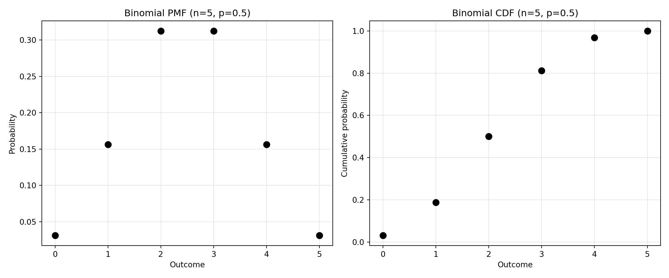
The following visualization is dynamic, updating the plot of the probabilities as \(N\) and \(p\) are changed. Drag \(N\) and \(p\) to the left and right to change the plot.
6.3.2 Special functions: PMF and CPF
- The function of \(P(X=x)\) is called the probability mass function or PMF.
- The function \(P(X\leq x)\) is called the cumulative probability function or probability function or CPF.
Often, when expressing the function mathematically, a lowercase letter, often \(f\), is used for the PMF and an uppercase letter, often \(F\) is used for the CPF.
For the binomial random variable, the PMF is
\[f(x) = P(X = x) = {N \choose x}p^x(1-p)^{N-x}\]
The probability function is
\[F(x) = P(X \leq x) = \sum_{u=0}^x{N \choose u}p^u(1-p)^{N-u}\]
The following section shows the derivation of the formula for the binomial probability mass function.
Derivation of binomial formula
6.3.3 How to calculate the probability of a sequence (order matters)?
Because successive outcomes are independent and \(p\) is constant,
\[ \begin{align*}P(1,\ 0,\ 1,\ 1,\ 1,\ 0) &= P(1)P(0)P(1)P(1)P(1)P(0) \\ & = p(1-p)ppp(1-p) \\ & = p^4(1-p)^2 \end{align*} \]
6.3.4 What about when order doesn’t matter?
- How do we calculate P(2 heads in 4 flips)?
- If the sequence was \(H,\ H,\ T,\ T\), then \[P(H,\ H,\ T,\ T) = p^2(1-p)^2\]
- If the sequence was \(T,\ T,\ H,\ H\), then \[P(T,\ T,\ H,\ H) = p^2(1-p)^2\]
- We could list all possible 4 flip sequences …

- How do we calculate P(2 heads in 4 flips)?
- We could list all possible 4 flip sequences …
- Identify all the sequences that have 2 heads …

- How do we calculate P(2 heads in 4 flips)?
- We could list all possible 4 flip sequences …
- Identify all the sequences that have 2 heads …
\[ \begin{align*}P(\text{2 heads}\ & \text{in 4 flips}) =\\ P(&\text{HHTT or HTHT or HTTH or} \\ &\text{THHT or THTH or TTHH})\end{align*} \]
- How do we calculate P(2 heads in 4 flips)?
- We could list all possible 4 flip sequences …
- Identify all the sequences that have 2 heads …
- Because the sequences are mutually exclusive:
\[\begin{align*}P(\text{2 heads in 4 flips}) &= P(HHTT)\\& + P(HTHT)\\& + P(HTTH)\\& + P(THHT)\\& + P(THTH)\\& + P(TTHH) \end{align*}\]
\[\begin{align*}P(\text{2 heads in 4 flips}) &= p^2(1-p)^2\\& + p^2(1-p)^2\\& + p^2(1-p)^2\\& + p^2(1-p)^2\\& + p^2(1-p)^2\\& + p^2(1-p)^2 \end{align*}\]
\[P(\text{2 heads in 4 flips}) = 6\ p^2(1-p)^2\]
6.3.4.1 Generally (for arbitrary N)
- How do we calculate \(P(X \text{ heads in } N \text{ flips})\)?
\[ \begin{align*}P(X &\text{ heads in } N \text{ flips}) = \\ &\text{[Number of sequences with X heads]} \times p^X(1-p)^{N-X}\end{align*} \]
\[P(X \text{ heads in } N \text{ flips}) = {N \choose X} p^X(1-p)^{N-X}\]
6.3.5 Binomial random variable PMF and CPF in Python
from scipy.stats import binom
import numpy as np

# Probability 2 heads in 4 flips when p = 0.5
binom.pmf(2, 4, 0.5)
# Probability 2 or fewer heads in 4 flips when p = 0.5
binom.cdf(2, 4, 0.5)
# Pseudo-random draw of the number of heads in 10 flips when p = 0.75
np.random.binomial(n=10, p=0.75, size = 1)
binom.rvs(n=10, p=0.75, size=1)
np.float64(0.375)
np.float64(0.6875)
array([6], dtype=int32)
array([5])6.4 Negative Binomial
Suppose one flips a coin until there are 5 heads
- HHHHH
- HTTHHTH
- TTTTHTTTHTTTHTTHH
- …
The number of failures before the \(K^{th}\) success in a Bernoulli sequence is a negative binomial random variable
Bernoulli properties still apply: independent outcomes, constant probability
Notation:
- \(p\) = probability of success in a single Bernoulli replicate
- \(K\) = number of successes in Bernoulli sequence
What are the possible values?
- 0, 1, 2, 3, …
6.4.1 Negative binomial PMF and CPF
\[ P(X = x) = {x + K - 1 \choose x}p^{K}(1-p)^{x} \]
\[ P(X \leq x) = \sum_{u=0}^x{u + K - 1 \choose u}p^{K}(1-p)^{u} \]
How to derive the PMF of a negative binomial random variable
What is P(3 tails before 5th head)?
- [3 tails before 5th head] = [hand of 3 tails and 4 heads] and [heads]
\[\text{P[hand of 3 tails and 4 heads] P[heads]}\]
\[{7 \choose 3}p^4(1-p)^3 \times p = {7 \choose 3}p^5(1-p)^3\]
In general, the negative binomial PMF can be expressed as a function of the binomial PMF
nbinom.pmf(x, k, p) = binom.pmf(x, k+x-1, p) * p6.4.2 Negative binomial PMF and CPF in Python
from scipy.stats import nbinom
import numpy as np

# Probability 2 failures before 5th success when p = .4: P(X = 2|K=5, p=0.4)
nbinom.pmf(2, 5, 0.4)
# Probability or 2 or fewer failures before 5th success when p = .4: P(X ≤ 2|K=5, p=0.4)
nbinom.cdf(2, 5, 0.4)
# Pseudo-random draw of the number of failures before 5th success when p = 0.4
nbinom.rvs(5, p=0.4, size=1)
np.float64(0.05529600000000003)
np.float64(0.09625600000000005)
array([3])6.4.3 Visualization of negative binomial PMF and CPF in Python
Code
import numpy as np
import matplotlib.pyplot as plt
from scipy.stats import nbinom

k = 5
p = 0.25
x = np.arange(0, 50)

fig, (ax1, ax2) = plt.subplots(1, 2, figsize=(12, 5))

pmf = nbinom.pmf(x, k, p)
ax1.plot(x, pmf, 'o', markersize=8, color='black')
ax1.set_xlabel('Outcome')
ax1.set_ylabel('Probability')
ax1.set_title('Neg Binomial PMF (k=5, p=0.25)')
ax1.grid(True, alpha=0.3)

cdf = nbinom.cdf(x, k, p)
ax2.plot(x, cdf, 'o', markersize=8, color='black')
ax2.set_xlabel('Outcome')
ax2.set_ylabel('Cumulative probability')
ax2.set_title('Neg Binomial CDF (k=5, p=0.25)')
ax2.grid(True, alpha=0.3)

plt.tight_layout()
plt.show()
In the interactive plot, you can observe how the PMF changes as \(p\) and \(K\) change.
6.5 Poisson random variable
The last random variable in this chapter is the poisson which is related to Bernoulli trials and the binomial distribution.
![]()
6.5.1 In teaching lore
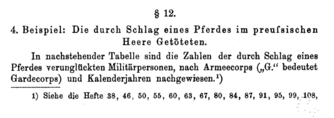
6.5.1.1 In teaching lore … the death by horse kick distribution
![]()
In general, the Poisson distribution is useful for describing the number of events that occur during a specified time interval.
6.5.2 Examples of data that might be described by a Poisson distribution
From a Pubmed search for articles.


6.5.3 Poisson PMF
\[ P(X = x|\lambda) = \frac{\lambda^xe^{-\lambda}}{x!} \]
\[\lambda = \text{Controls the rate of events}\]
6.5.4 Poisson CDF
\[ P(X \leq x|\lambda) = \sum_{u=0}^x\frac{\lambda^ue^{-\lambda}}{u!} \]
6.5.5 Poisson PMF and CPF in Python
from scipy.stats import poisson

# Probability 4 crashes today on a stretch of I-64 if lambda = 2
poisson.pmf(k=4, mu=2)

# Probability 4 or fewer crashes today on a stretch of I-64
poisson.cdf(k=4, mu=2)

# Pseudo-random draw of the number of crashes today on a stretch of I-64
poisson.rvs(mu=2, size=1)
np.float64(0.09022352215774178)
np.float64(0.9473469826562889)
array([2])6.5.6 Visualizations of Poisson PMF and CPF
Code
import numpy as np
import matplotlib.pyplot as plt
from scipy.stats import poisson

l = 2
x = np.arange(0, 10)

fig, (ax1, ax2) = plt.subplots(1, 2, figsize=(12, 5))

pmf = poisson.pmf(x, l)
ax1.plot(x, pmf, 'o', markersize=8, color='black')
ax1.set_xlabel('Outcome')
ax1.set_ylabel('Probability')
ax1.set_title('Poisson PMF (lambda = 2)')
ax1.grid(True, alpha=0.3)

cdf = poisson.cdf(x, l)
ax2.plot(x, cdf, 'o', markersize=8, color='black')
ax2.set_xlabel('Outcome')
ax2.set_ylabel('Cumulative probability')
ax2.set_title('Poisson CDF (lambda = 2)')
ax2.grid(True, alpha=0.3)

plt.tight_layout()
plt.show()
In the dynamic plot below, you can see how the PMF changes as \(\lambda\) changes. Drag \(\lambda\) to the left or right.
6.5.7 Interpreting \(\lambda\)
The parameter \(\lambda\) is the event rate; it is the number of events per period time. For example, if the number of charitable donations per year follows a Poisson distribution, then \(\lambda = 5\) would suggest that on average, 5 charitable donations are recieved every year.
6.5.8 Changing the time scale of a Poisson outcome
The Poisson distribution has a special property that allows easy modification of the time scale.
\[ \begin{array}{rl} \text{If } X &=\text{number of charitable donations per year}\\ \text{and } X &\sim \text{POISSON}(\lambda = 5)\\ \text{then the number of charitable donations per decade} &\sim \text{POISSON}(\lambda = 5\times 10)\\ \text{or the number of charitable donations per month} &\sim \text{POISSON}\left(\lambda = 5\times \frac{1}{12}\right)\\ \end{array} \]
This allows for easy calculation of the probability of events on a different time scale.
\[P(\text{Charitable donations in a decade} = 50) = \text{poisson.pmf(50, 5*10)}\]
from scipy.stats import poisson
poisson.pmf(50, 5*10)
6.6 Practice problems
- A hospital emergency room receives an average of 4.5 patients per hour. What is the probability that exactly 6 patients arrive in a given hour?
- A basketball player has a 65% free throw success rate. If she attempts 12 free throws in a game, what is the probability she makes exactly 8 of them?
- A salesperson has a 20% chance of making a sale with each customer contact. What is the probability that they will need to contact exactly 15 customers before achieving their 4th sale?
- Typing errors occur in a manuscript at an average rate of 2.5 errors per page. What is the probability of finding exactly 4 errors on a randomly selected page?
- In a multiple-choice test with 10 questions, each question has 4 options. If a student guesses randomly on all questions, what is the probability they get exactly 3 correct answers?
- A oil company drills wells with a 25% success rate. What is the probability they drill exactly 8 wells before finding their 2nd productive well?
- A quality control inspector finds that 15% of items from a production line are defective. If she randomly selects 20 items, what is the probability that at most 2 are defective?
- Cars pass through a toll booth at an average rate of 8 vehicles per minute. What is the probability that exactly 10 cars pass through in a given minute?
- A archer hits the bullseye 30% of the time. What is the probability that she will need exactly 10 shots to hit her 3rd bullseye?
- A call center receives an average of 3 customer complaints per day. What is the probability they receive no complaints on a particular day?