import numpy as np
from itertools import groupby
import matplotlib.pyplot as plt
import pandas as pd

def oneplay(B=200, W=300, L=200, M=100, summary = True):

    # martingale
    def wager(ledger):
        if ledger["outcome"][-1] == 1:
            new_wager = 1
        else:
            new_wager = min(2*ledger["wager"][-1], M, ledger["budget"][-1])
        ledger["wager"].append(new_wager)

    def spin(ledger):
        spin = np.random.binomial(1, p = 18/38)
        ledger["outcome"].append(spin)

    def stop_rule(ledger):
        if ledger["outcome"][-1] == 1:
            ledger["budget"].append(ledger["budget"][-1] + ledger["wager"][-1])
        else:
            ledger["budget"].append(ledger["budget"][-1] - ledger["wager"][-1])

        if ledger["budget"][-1] >= W:
            outcome = 1
        elif len(ledger["budget"]) - 1 >= L:
            outcome = -1
        elif ledger["budget"][-1] <= 0:
            outcome = -2
        else:
            outcome = 0
        return outcome

    # ledger
    ledger = {"budget":[B, B], "wager":[0], "outcome":[1]}
    outcome = 0
    while outcome == 0:
        wager(ledger)
        spin(ledger)
        outcome = stop_rule(ledger)

    if summary == False:
        return ledger

    bad_luck = max([len(list(values)) for key, values in groupby(ledger["outcome"]) if key == 0])

    summary = {
          "B":B
        , "W":W
        , "L":L
        , "M":M
        , "outcome":outcome
        , "profit":ledger["budget"][-1] - B
        , "n_games":len(ledger["budget"]) - 1
        , "prop_red":np.mean(ledger["outcome"])
        , "bad_luck_streak": bad_luck
    }

return summaryRoulette and the martingale betting strategy
In this deliverable, you are going to use simulation to evaluate the profitability of a well-known betting strategy. Watch (in double speed) the following clip for a video introduction to roulette and the martingale betting strategy.
Roulette basics
A roulette table composed of 38 (or 37) evenly sized pockets on a wheel. The pockets are colored red, black, or green. The pockets are also numbered. Roulette is a game of chance in which a pocket is randomly selected. Gamblers may wager on several aspects of the outcome. For example, one may place a wager that the randomly selected pocket will be red or odd numbered or will be a specific number.
For this assignment, all one needs to know is that there are 38 pockets of which 2 are green, 18 are red, and 18 are black. The payout for a bet on black (or red) is $1 for each $1 wagered. This means that if a gambler bets $1 on black and the randomly selected pocket is black, then the gambler will get the original $1 wager and an additional $1 as winnings.
Roulette betting strategies
There are several strategies for playing roulette. (Strategies is in italics because the house always wins, in the long run.) Consider one such strategy:

This is a classic roulette strategy called the “Martingale” strategy. Consider how the strategy playes out for a single sequence of spins {Black, Black, Red}.
| Play | Wager | Outcome | Earnings |
|---|---|---|---|
| 1 | 1 | Black | -1 |
| 2 | 2 | Black | -3 |
| 3 | 4 | Red | +1 |
Now consider a sequence {Black, Black, Black, Red}.
| Play | Wager | Outcome | Earnings |
|---|---|---|---|
| 1 | 1 | Black | -1 |
| 2 | 2 | Black | -3 |
| 3 | 4 | Black | -7 |
| 4 | 8 | Red | +1 |
The Martingale strategy appears to always end in positive earnings, regardless of how unlucky a string of spins may be. Is the strategy actually profitable?
Assignment
In this assignment, you will write a blog post to explain how you used computer simulation to understand the profitability of the above strategy.
The audience of your blog post is a sharp college freshman with little to no background in data science.
You should explain how you used computer simulation to calculate the average earnings of a gambler that uses this strategy. As part of the explanation, provide a figure (or a series of figures) that show how the gamblers earnings (or losses) evolve over a series of wagers at the roulette wheel. (The x-axis will be the wager number (or play number), the y-axis will be available budget.)
Show your audience how changing a parameter of the simulation (see table below) does or does not have an impact on average profit. Create a figure to show the impact.
Be sure to end with a take home message that answers the main question: Is the strategy actually profitable?.
Blog posts tend to be less formal than academic reports. Feel free to include figures, gifs, memes, or videos that help the reader engage with the topic and your explanation.
Submission instructions
- Create an html blog post with Quarto or Jupyter notebooks.
- Be prepared to share your blog post with your classmates when the deliverable is due.
- The deliverable should be your own work.
- Make sure the your code is viewable, and print the html report to PDF for submission to GradeScope.
- Submit the PDF report to GradeScope via Canvas (link)
Simulation setup
As noted in the video introduction, there are a few settings or conditions that we need to set for the simulation. These are simulation parameters.
Stopping rule
A player will use the above strategy and play until
- the player has W dollars
- the player goes bankrupt
- the player completes L spins (or wagers or plays)
Budget
The player starts with B dollars. The player cannot wager more money than he/she has.
Maximum wager
Some casinos have a maximum bet. Call this parameter M. If the strategy directs the player to wager more than M dollars, then the player will only wager M dollars.
Summary of parameters
| Parameter | Description | Starting value |
|---|---|---|
| B | Starting budget | $200 |
| W | Winnings threshold for stopping | $300 (Starting budget + $100 winnings) |
| L | Time threshold for stopping | 200 plays (roughly 5 to 6 hours) |
| M | Casino’s maximum wager | $100 |
Code
Here is the video recording of the live coding. As always, watch in double or triple speed.
The final form of the code is below.
Simulation of 5 visits to the casino
Here, we generate a plot of the losses and gains of 5 simulated visits to the casino. The simulation uses the default parameter values.
np.random.seed(20250925) # DO NOT USE THE SAME SEED FOR YOUR DELIVERABLE
plt.close()
for i in range(5):
    p1 = oneplay(summary = False)
    plt.plot(p1["budget"])
plt.ylim([-10, 310])
plt.xlabel("Spin number")
plt.ylabel("Budget")
plt.show()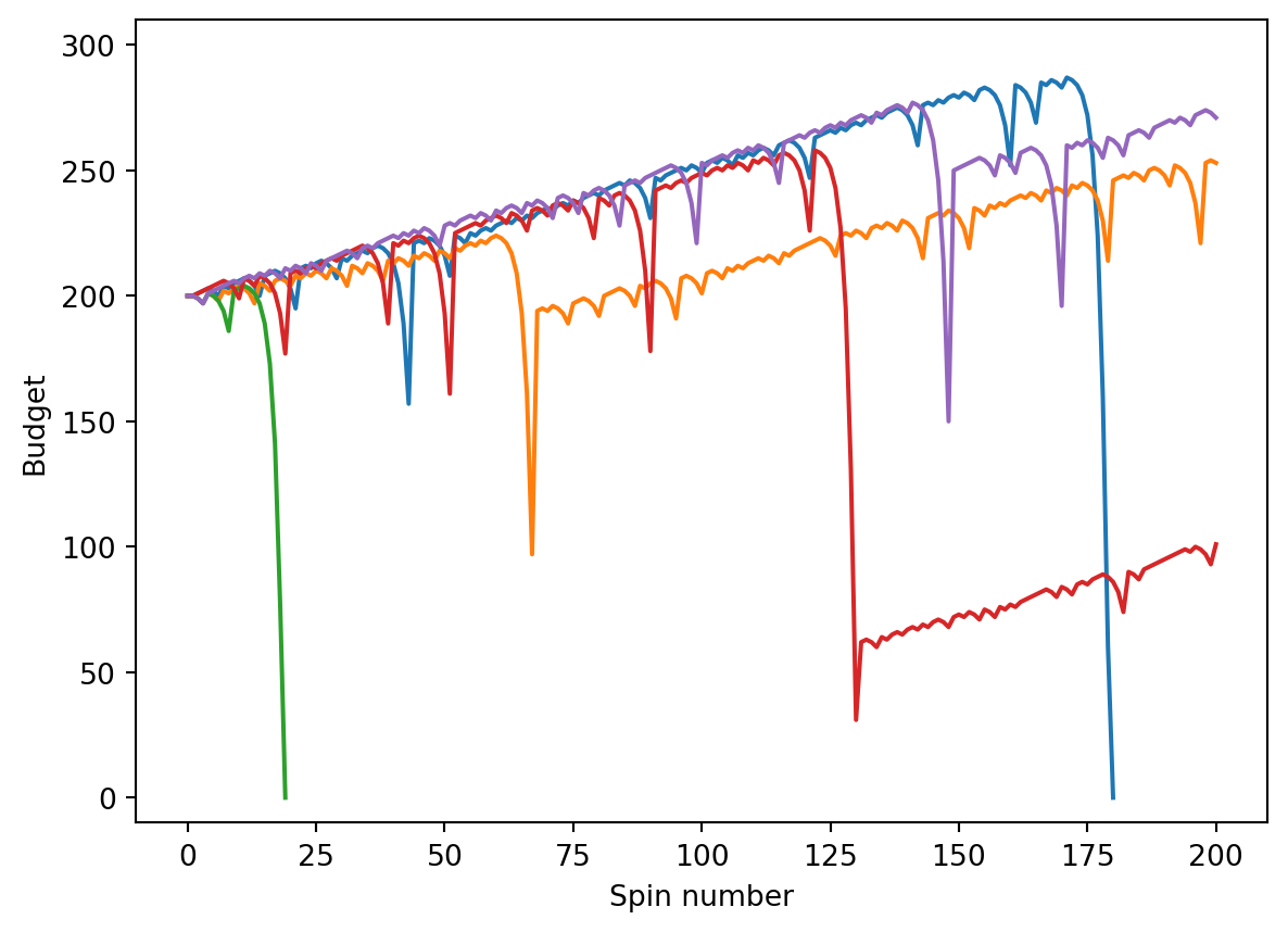
Two of the simulations resulted in bankruptcy and a third lost money. Two won some money but had to stop before reaching the $300 goal because they ran out of time.
Average profit over 10,000 visits
Here simulate the martingale strategy 10K times, calculating the average profit.
R = 10000
A = [oneplay() for i in range(R)]
B = pd.DataFrame(A)
B.profit.mean().item()-36.5704We see average losses of -36.5704 under the default simulation parameters.
Average profit for different winning thresholds
Here we calculate the average profit for several winning thresholds.
R = 40000
A = [oneplay(W = 200 + j) for j in [25, 50, 75, 100, 125, 150] for i in range(R)]
B = pd.DataFrame(A)
C = B.pivot_table(values="profit", index = "W").reset_index()
plt.close()
C.assign(walk_away_rule = C.W - 200).plot(x="walk_away_rule", y = "profit", legend = False)
plt.xlabel("Winning threshold")
plt.ylabel("Average profit")
plt.show()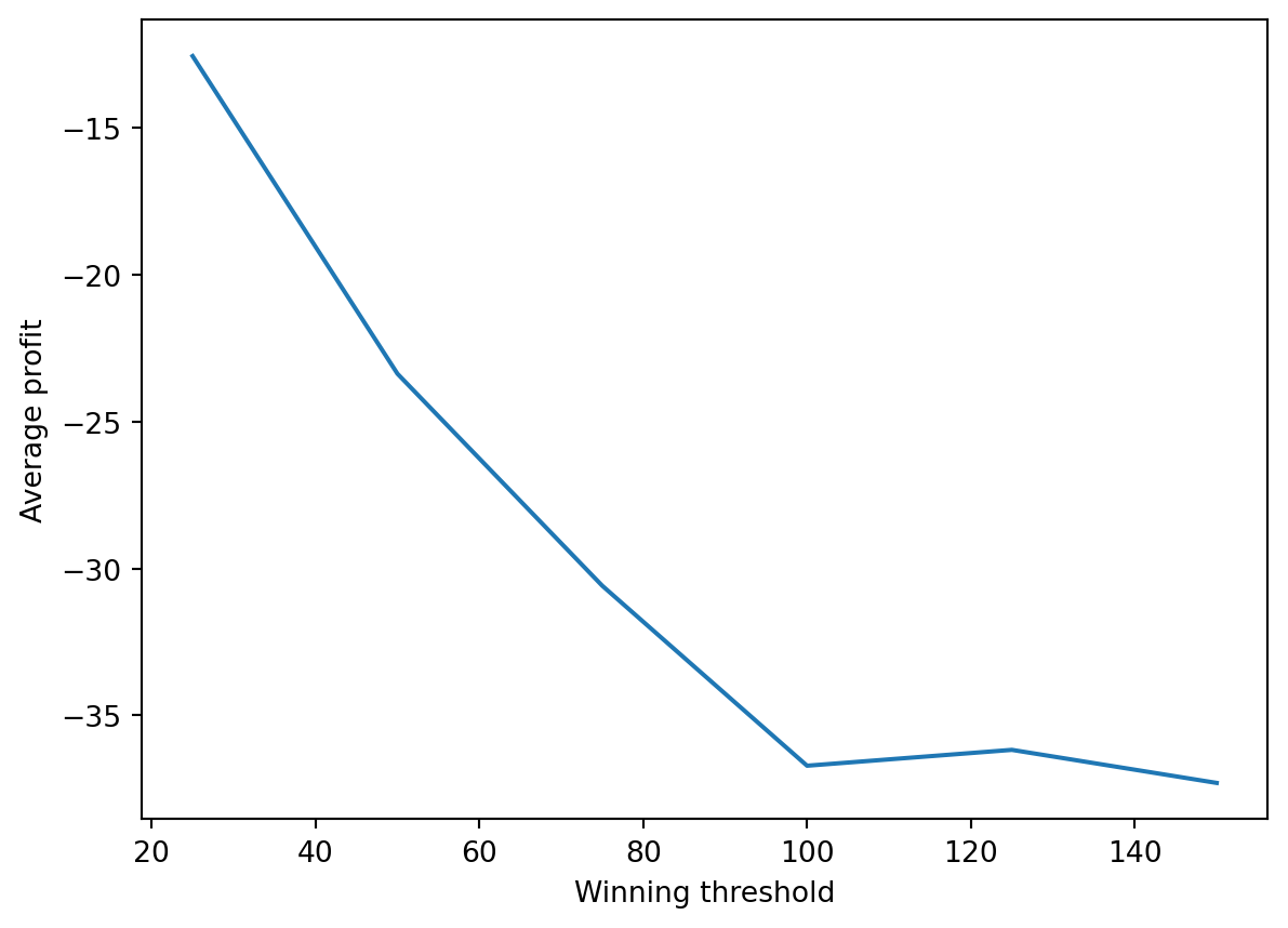
The main message is that average profit is negative for every winning threshold we considered. On average, the casino wins.