flowchart TB
A[Data types]
A --> B[Discrete]
A --> C[Continuous]
subgraph "This slide deck"
D["<p style='text-align:left;'>Probability\n+ Long-run proportion\n+ AND a ∩ b \n+ OR a ∪ b\n+ IN x ∈ {a,b,c}\n+ Conditional a|b\n+ Marginal\n+ PMF\n+ CPF (CDF)</p>"]
end
B --> D
D --> E["Examples of random variables"]
F["<p style='text-align:left;'>Balls from buckets\n+ Replacement (with or without)\n+ Order (Hand or sequence)</p>"]
E --> F
E --> G["<p style='text-align:left;'>Coin flips (weighted):\n+ Bernoulli (1 flip)\n+ Binomial (N flips)\n+ Neg Binomial (K successes)\n+ World Series (K successes or failures)</p>"]
E --> H["Events per period time\n+ Poisson"]
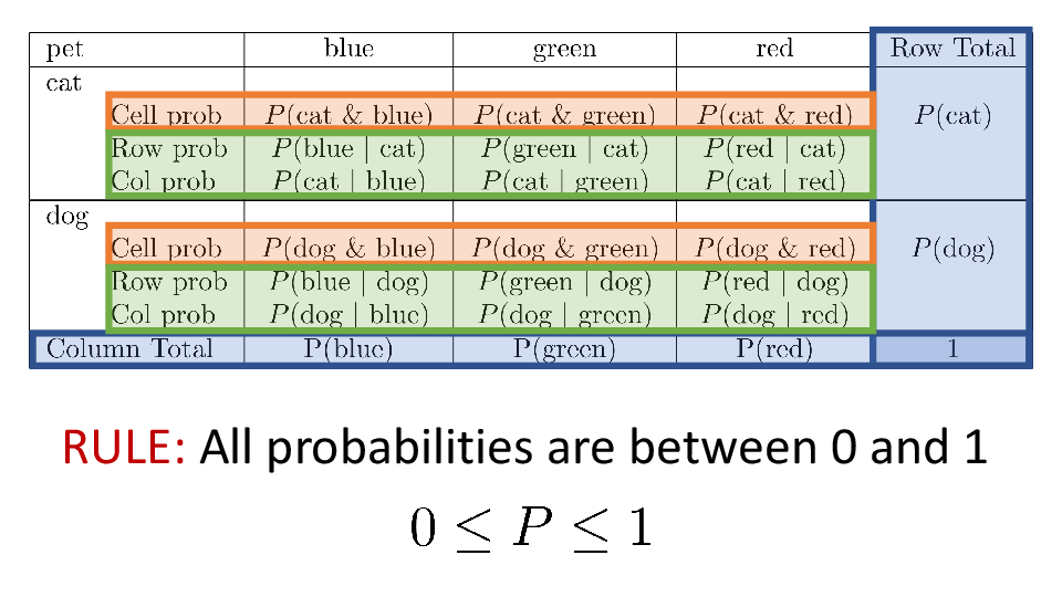
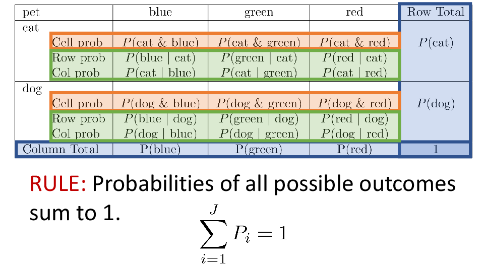
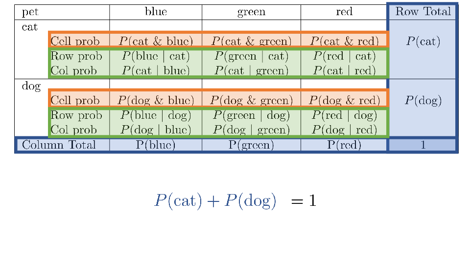
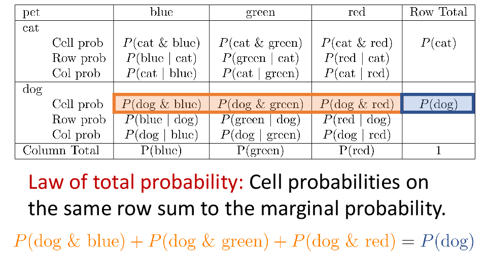
4 Rules of probability
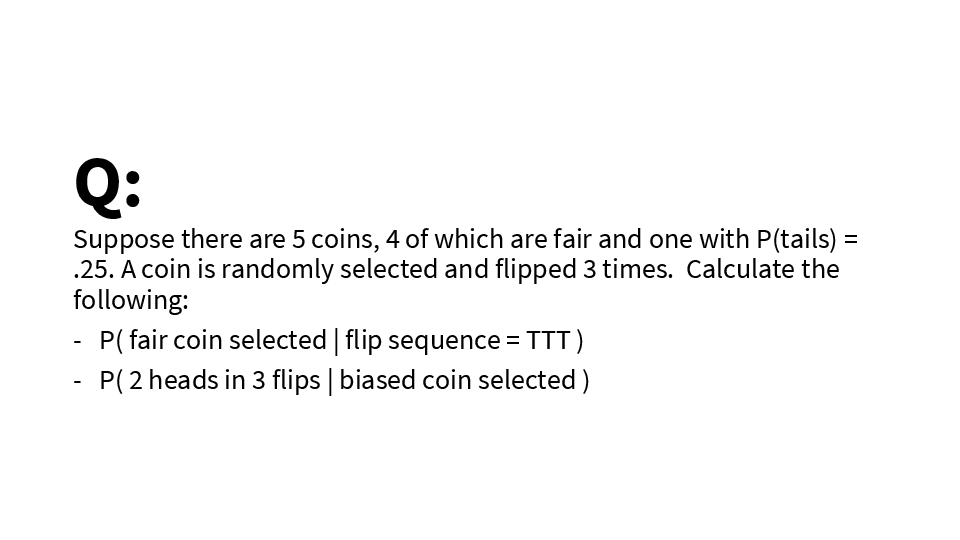
In the textbook and in class, we have talked about how the term probability has multiple definitions. Understanding these different definitions is crucial for correctly interpreting probability statements in various contexts. Consider what is meant by probability in the following examples.
In a class of 37 individuals, the probability that two students share a birthday is 0.84.
I think there is an 80% chance the defendant did the crime.
After performing the clinical trial, scientists reported a 0.98 probability that the treatment is effective.
Let’s examine what type of probability each example represents.
The first example uses probability to refer to a long-run proportion. Perhaps imagining thousands or millions of classrooms with 37 students, 0.84 refers to the proportion that have at least two students with the same birthday. This definition of probability is perhaps the definition that most individuals would offer when asked to define the word because it is the definition tied to games of chance, card games, and dice rolls.
The key elements of this definition are:
- Repeatable process
- Recordable outcome(s) from each execution or replicate of the process
- The proportion of replicates in which the outcome of interest is observed.
Let’s see how these elements apply to the poker example. Consider these key elements when someone says \[ \text{the probability of a royal flush is } \frac{1}{649740} \] in a game of 5-card stud poker. The repeatable process is shuffling a standard card deck and dealing 5 cards. The outcome of interest is whether or not the 5 cards are (a) all of one suit and (b) a straight from 10 to ace. Imagining the cards shuffled and dealt infinitely many times (or calculating this theoretically), the probability of the outcome (royal flush) is the proportion of deals which result in the outcome.
The second example with the defendant and a juror represents another way the word probability is used. In this example, the juror is probably not thinking of a repeatable process. Rather, they are in an uncertain situation, unable to conclusively state if the defendant did the crime. In this situation, the probability is an expression of belief or an expression of the degree of certainty/uncertainty in the defendant’s guilt. Interestingly, the juror uses the terminology from games of chance to express their degree of uncertainty. After hearing the evidence, the juror expresses their level of uncertainty by analogy to a game of chance, potentially imagining a bucket with 2 white balls representing “not guilty” and 8 black balls representing “guilty”. The juror’s uncertainty about the defendant’s guilt is comparable to the uncertainty associated with pulling a ball from the bucket.
The third example with the clinical trial is perhaps the most interesting. It represents an expression of belief updated by observed data. The researchers began with an initial belief about the efficacy of the drug. Effective drugs are rare, so it is likely the researchers began the trial skeptical, perhaps expressing their skepticism by analogy: “there is only a 1 in a 1000 chance the drug is effective”. However, as trial participants were enrolled and outcomes observed, the researchers updated their beliefs about the drug as the data accumulated. This example combines the expression of belief (as in the juror example) with the repeated observation of outcomes (as in the game of chance example). This represents a hybrid of the two definitions of probability, combining belief and observed data.
%%{init: {"flowchart": {"htmlLabels": false}} }%%
flowchart LR
  A["Long-run proportion"] <--> B["Expression of belief updated by observed data"] <--> C["Expression of belief"]
4.1 Probability as a long-run proportion
We start with probability as a long-run proportion. This is sometimes called the frequency definition of probability. It turns out that the rules for frequency probabilities will match the rules for expression of belief probabilities.
As noted in the previous section, the key elements of the frequency definition are:
- Repeatable process
- Recordable outcome(s) from each execution or replicate of the process
- The proportion of replicates in which the outcome of interest is observed.
We can think about the data frame of outcomes generated from this process. For example, the data frame below shows the outcome of a random process in which the outcomes are “species” and “color”.
| Species | Color | |
|---|---|---|
| 1 | virginica | purple |
| 2 | setosa | pink |
| 3 | versicolor | pink |
| ⋮ | ⋮ | |
| k | setosa | purple |
| k+1 | versicolor | pink |
| ⋮ | ⋮ |
To calculate the long-run proportion of an outcome, we need first calculate the proportion in the first \(N\) rows. First, we calculate the number of pink.
\[ \#(\text{pink}) = \sum_{i=1}^N I(\text{Color}_i = \text{pink}) \]
Note the use of \(I\), the indicator function, which is defined as
\[ I(x) = \left\{\begin{array}{ll} 1 & x\text{ is true} \\ 0 & \text{otherwise} \end{array} \right. \]
If we add a new column to our data frame for \(I(\text{Color}_i = \text{pink})\), it simply adds a column of ones and zeros.
| Species | Color | \(I(\text{Color}_i = \text{pink})\) | |
|---|---|---|---|
| 1 | virginica | purple | 0 |
| 2 | setosa | pink | 1 |
| 3 | versicolor | pink | 1 |
| ⋮ | ⋮ | ⋮ | |
| k | setosa | purple | 0 |
| k+1 | versicolor | pink | 1 |
| ⋮ | ⋮ | ⋮ |
The proportion of pink in the first N rows is
\[ \frac{\#(\text{pink})}{N} = \frac{1}{N}\sum_{i=1}^N I(\text{Color}_i = \text{pink}) \]
The frequency definition of probability is the limit of the proportion:
\[ P(\text{Color} = \text{pink}) = \lim_{N\to \infty} \frac{\#(\text{pink})}{N} \]
We can take the limit of any proportion that can be calculated from a finite data frame. Here are some other probabilities that might be meaningful.
\[ P(\text{Species starts with v}) \]
\[ P(\text{Setosa and pink}) \]
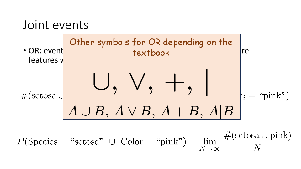
\[ P(\text{Setosa or pink}) \]
The trick is to use the indicator function \(I\) to find the rows that need to be counted in the numerator.
| Species | Color | \(I(\text{Color}_i = \text{pink})\) | \(I(\text{Species starts with v})\) | \(I(\text{Setosa and pink})\) | \(I(\text{Setosa or pink})\) | |
|---|---|---|---|---|---|---|
| 1 | virginica | purple | 0 | 1 | 0 | 0 |
| 2 | setosa | pink | 1 | 0 | 1 | 1 |
| 3 | versicolor | pink | 1 | 1 | 0 | 1 |
| ⋮ | ⋮ | ⋮ | ⋮ | ⋮ | ⋮ | |
| k | setosa | purple | 0 | 0 | 0 | 0 |
| k+1 | versicolor | pink | 1 | 1 | 0 | 1 |
| ⋮ | ⋮ | ⋮ | ⋮ | ⋮ | ⋮ |
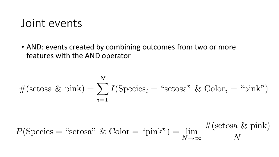
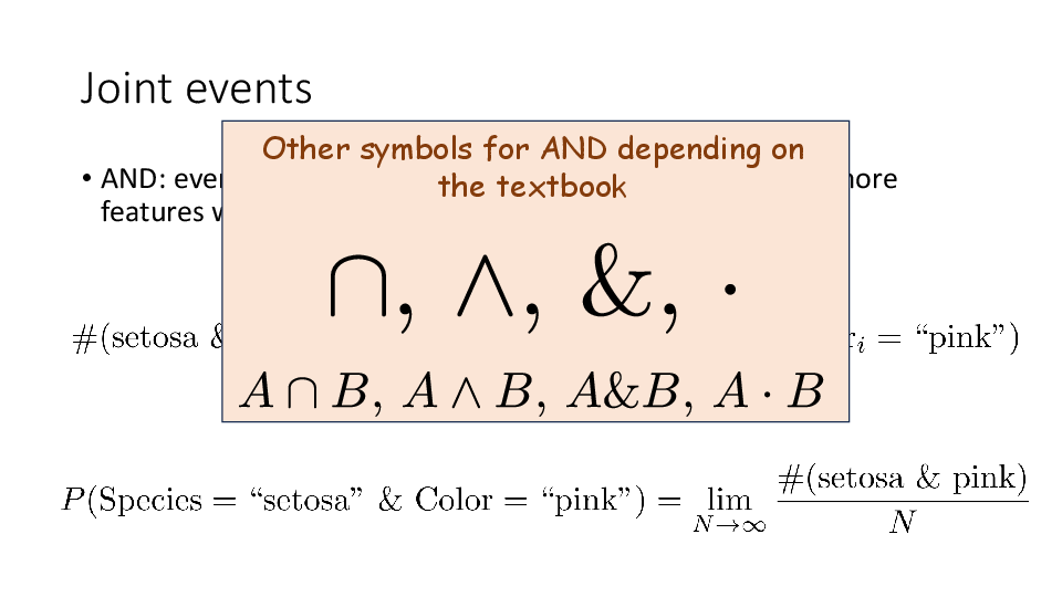
The event Setosa and pink is known as a joint event because it occurs when two outcomes occur jointly. In this case, the species is setosa simultaneously with color being pink.
This type of outcome is sometimes called an AND outcome because its definition uses the AND operator.
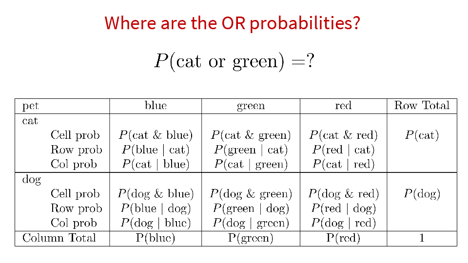
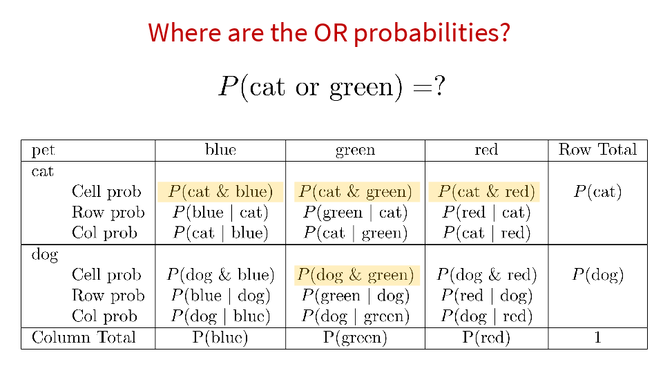
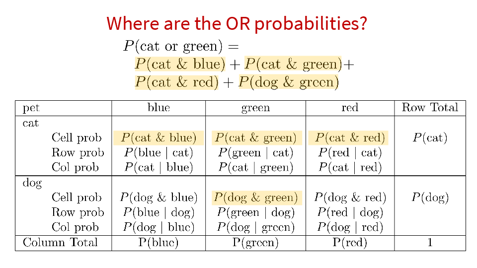
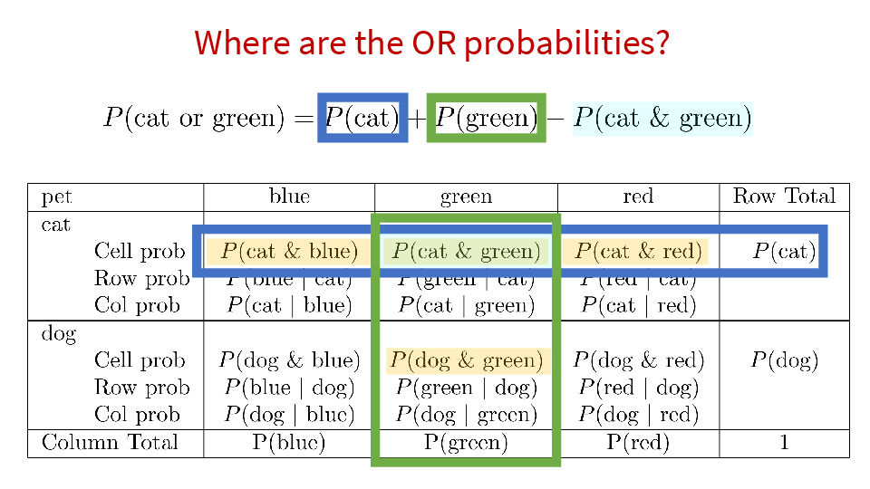
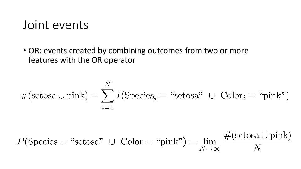
Just like events or outcomes can be defined with the AND opporator, events can also be defined with the OR operator. One might be interested in \(P(\text{Setosa or pink})\).
What type of outcome is Species starts with v? It is defined with only the Species outcome. It is an event that combines events of a single outcome.
\[ P(\text{Species starts with v}) = P(\text{Species} \in \{\text{versicolor}, \text{virginica} \}) \]
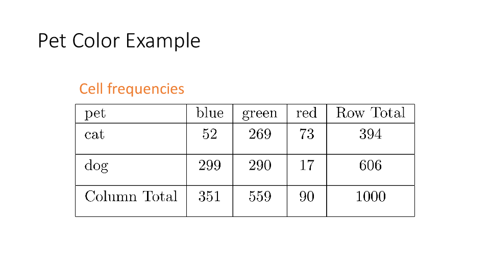
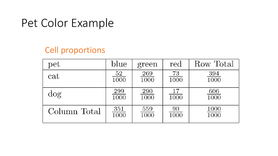
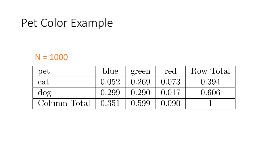
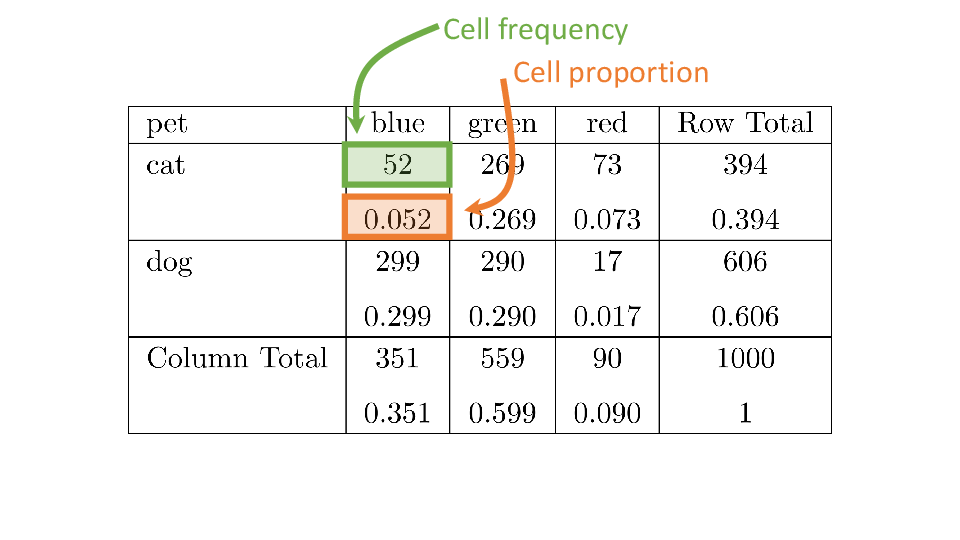
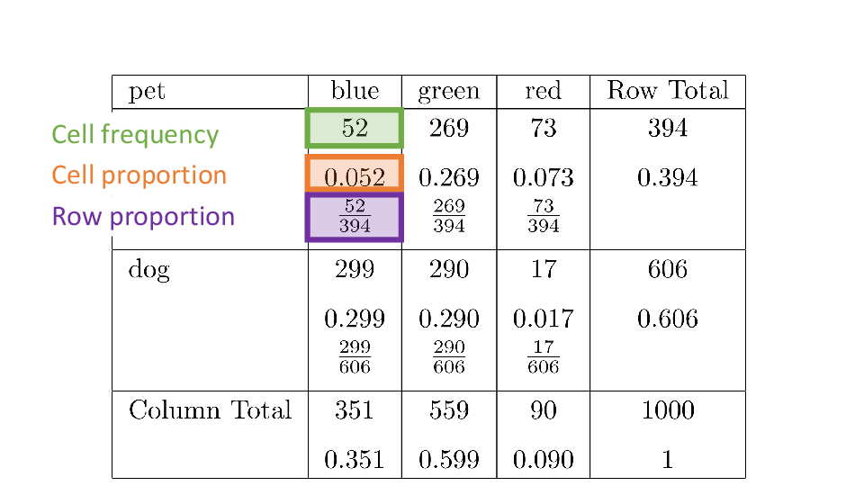
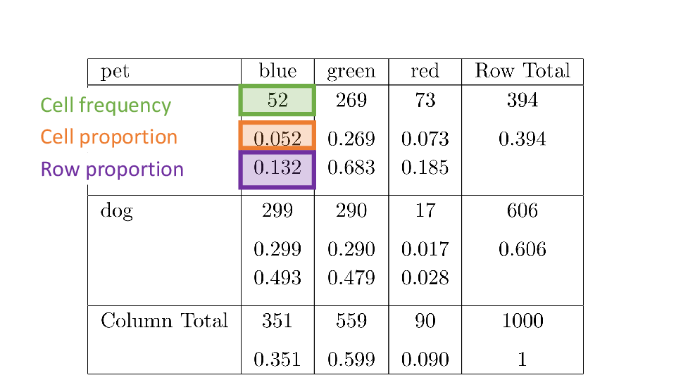
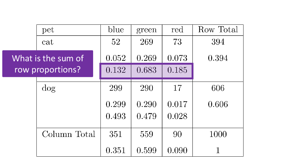
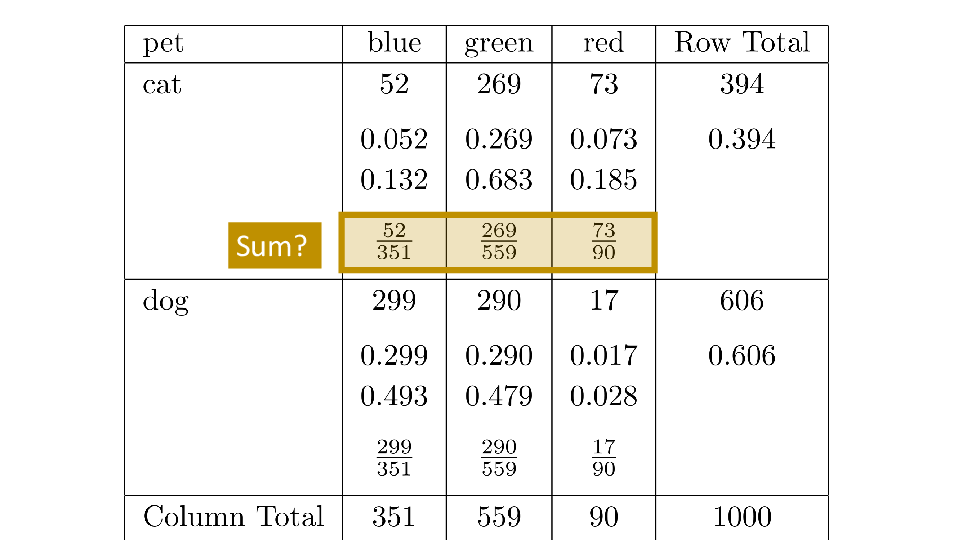
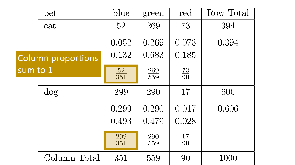
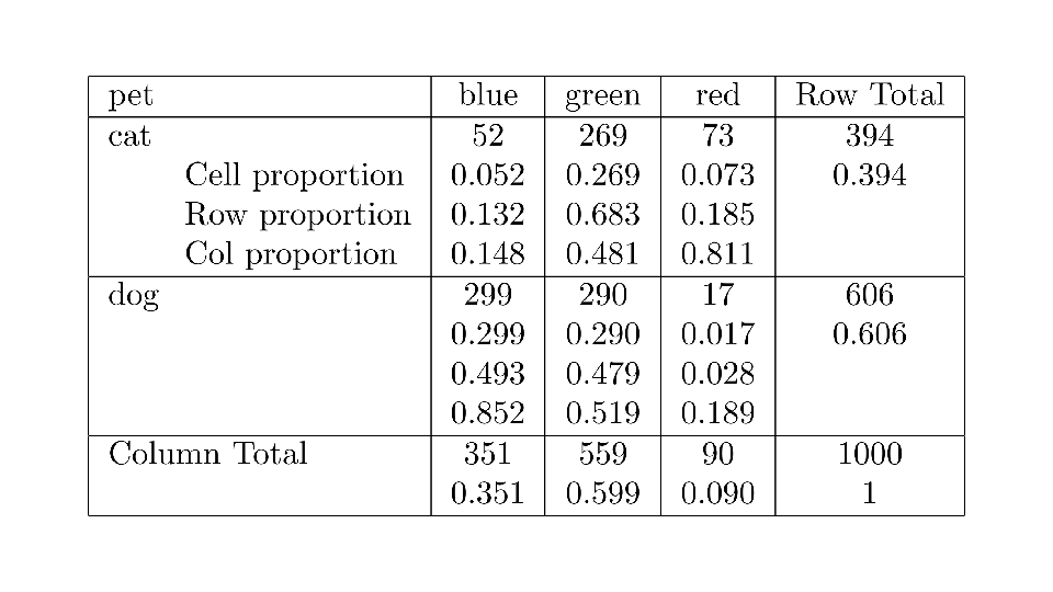
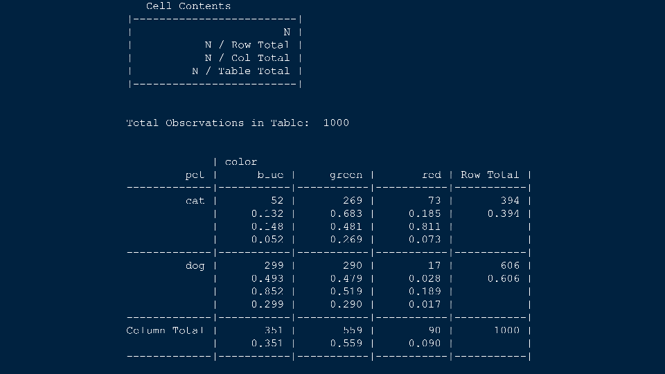
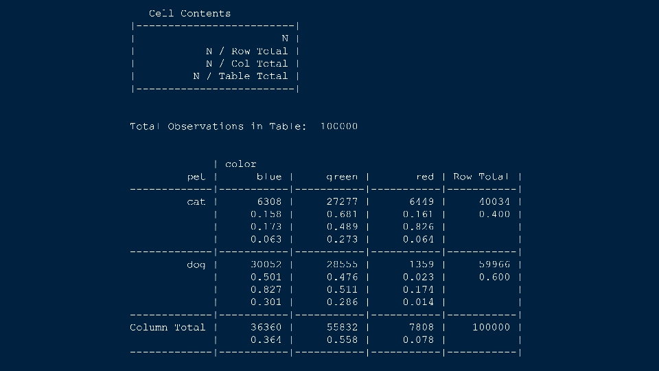
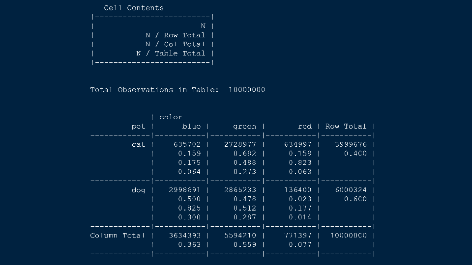
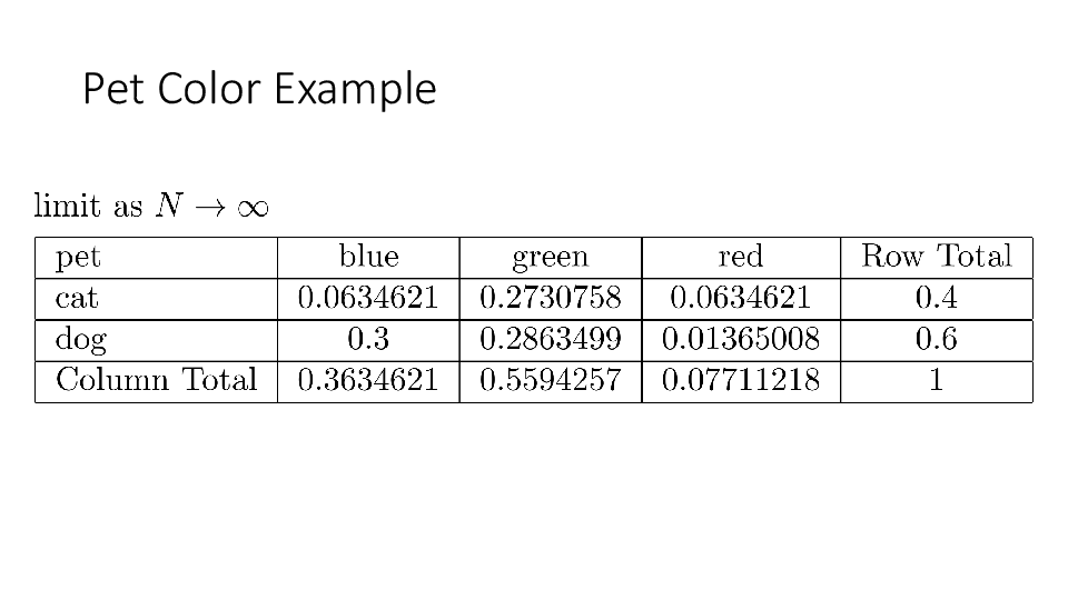
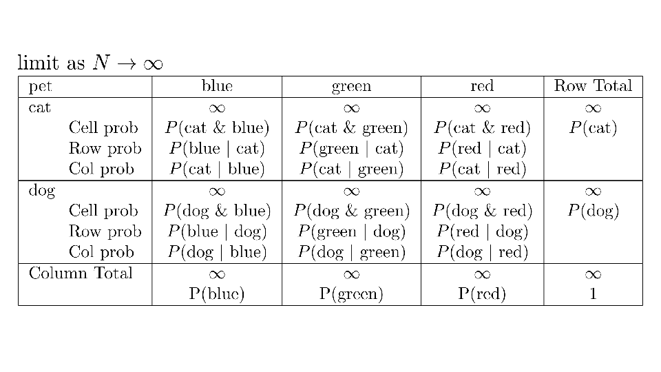
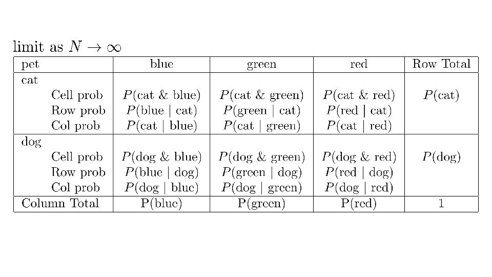
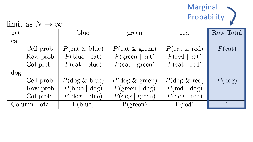
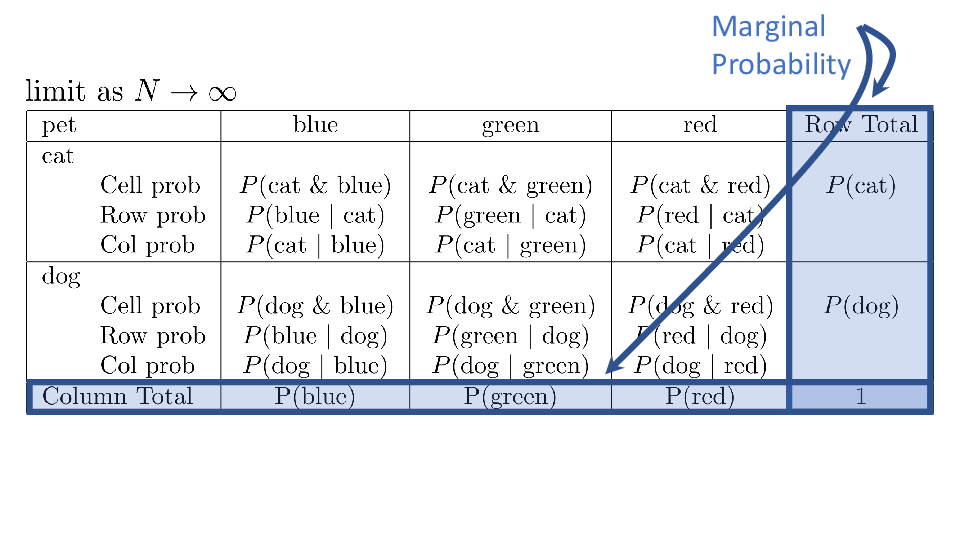
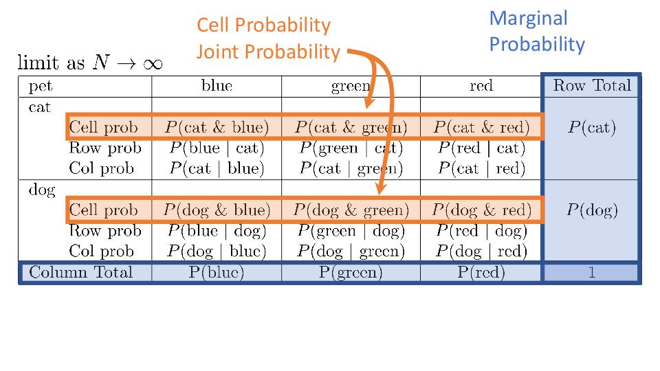
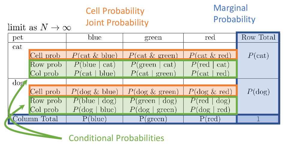
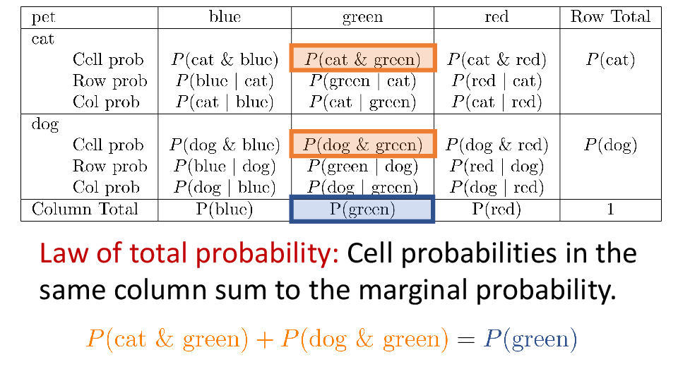
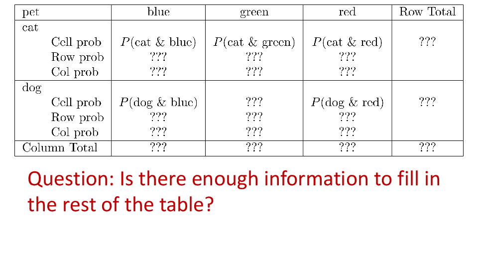
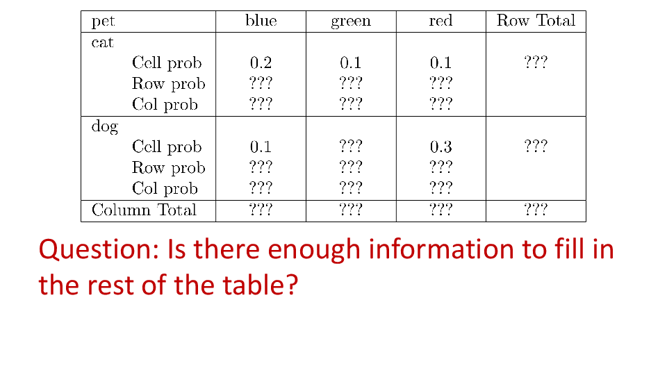
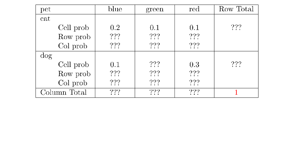
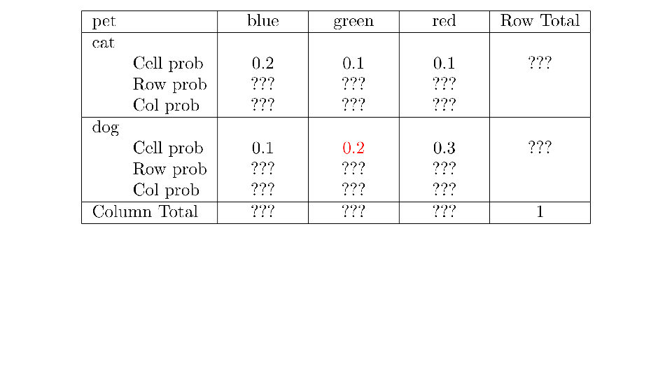
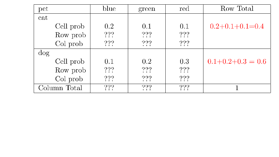
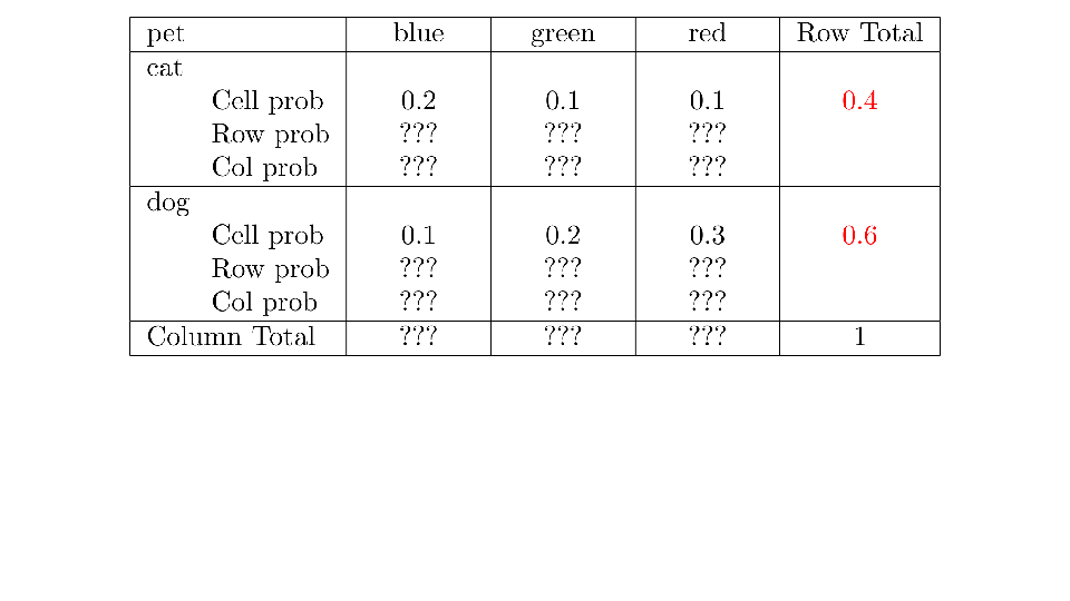
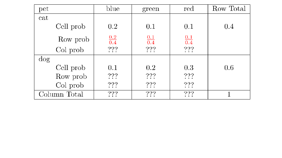
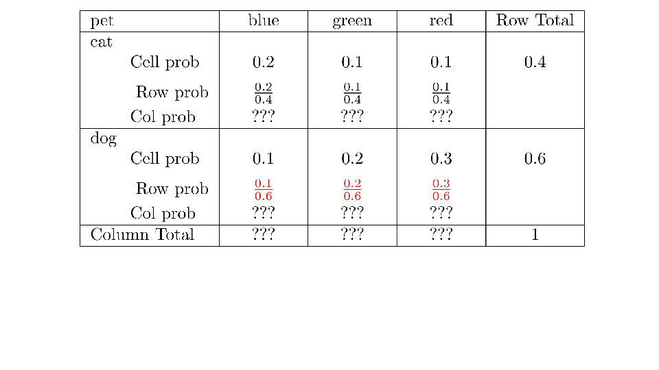
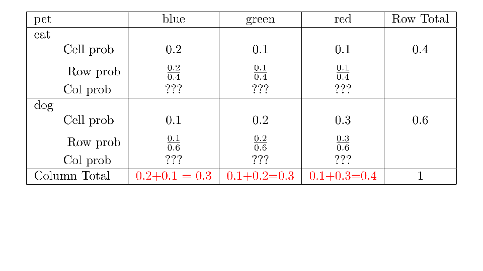
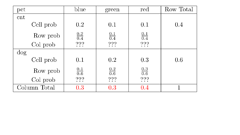
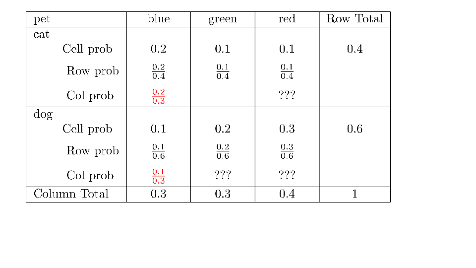
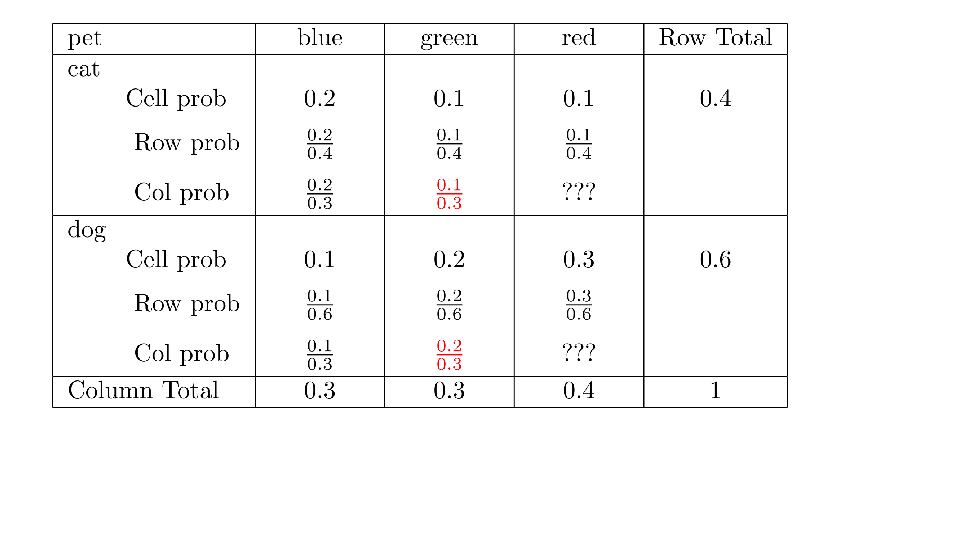
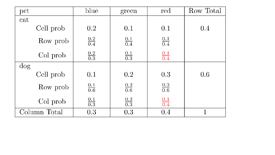
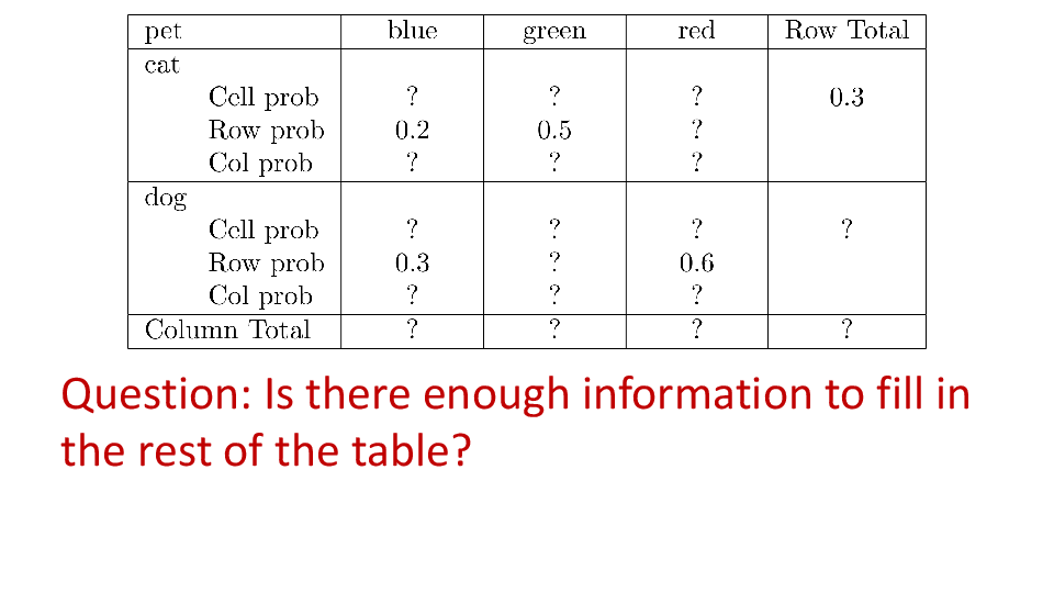
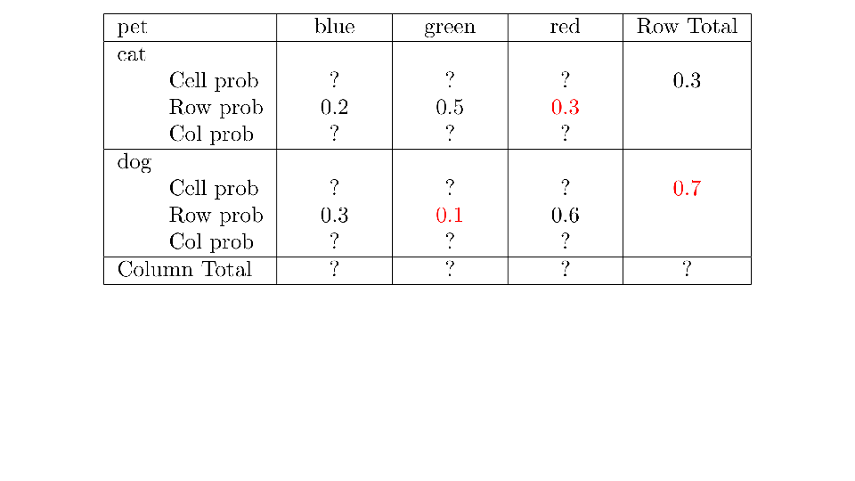
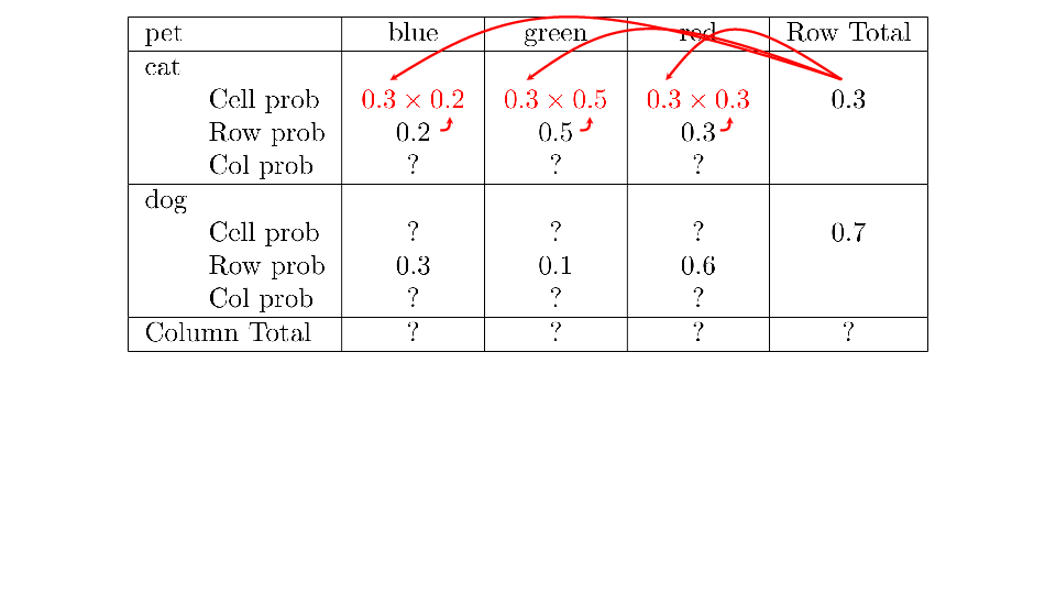
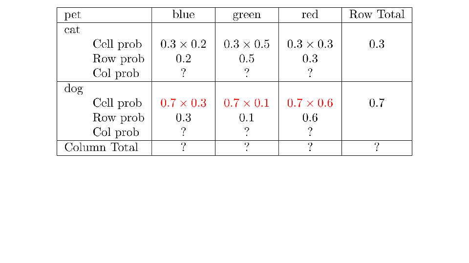
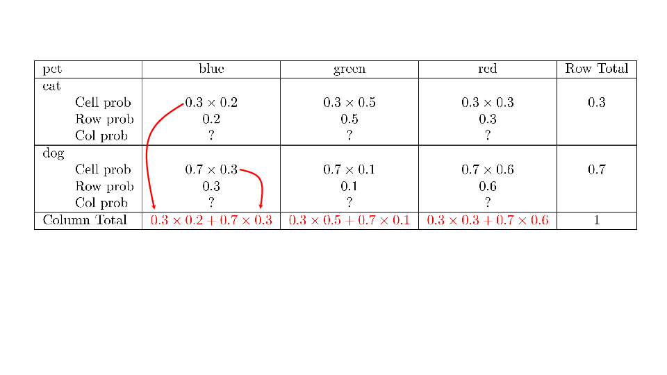
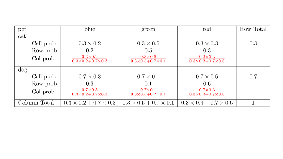
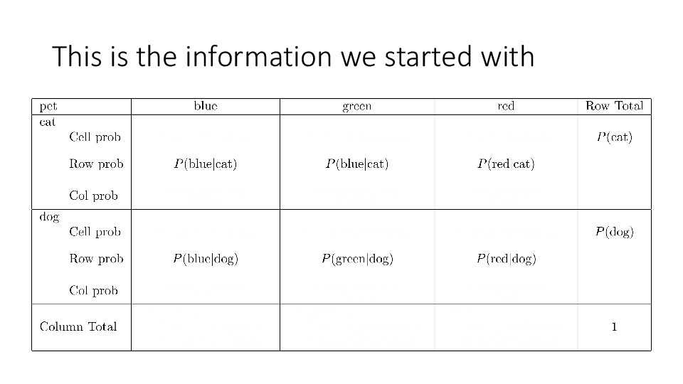
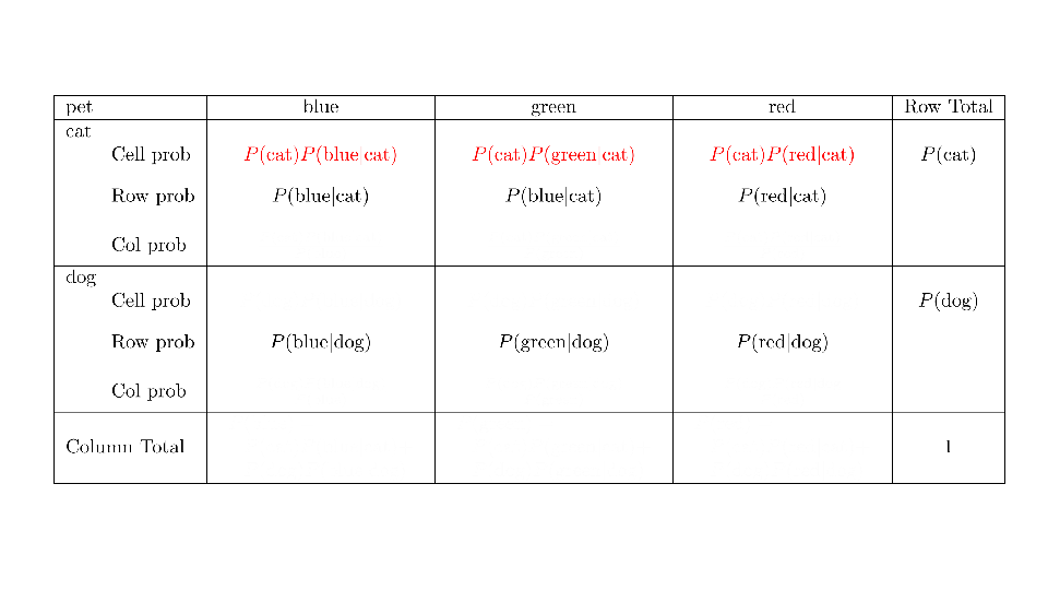
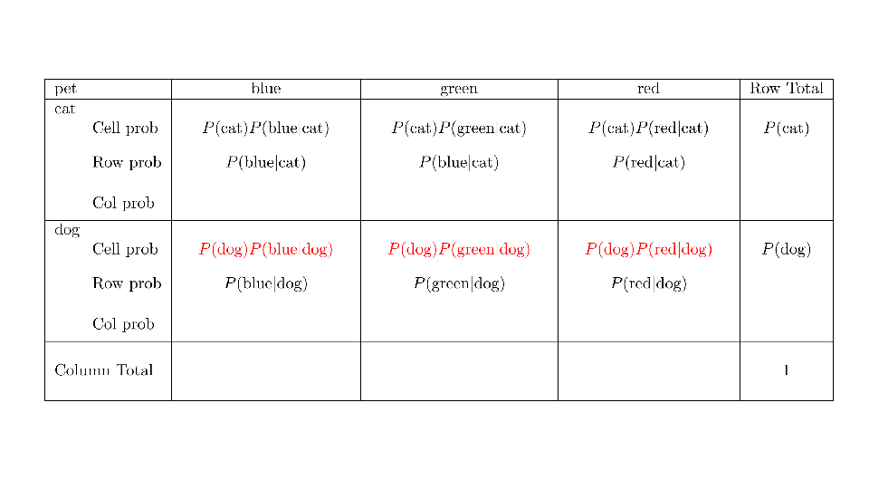
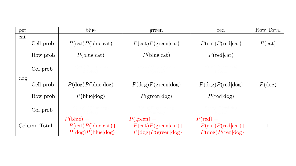
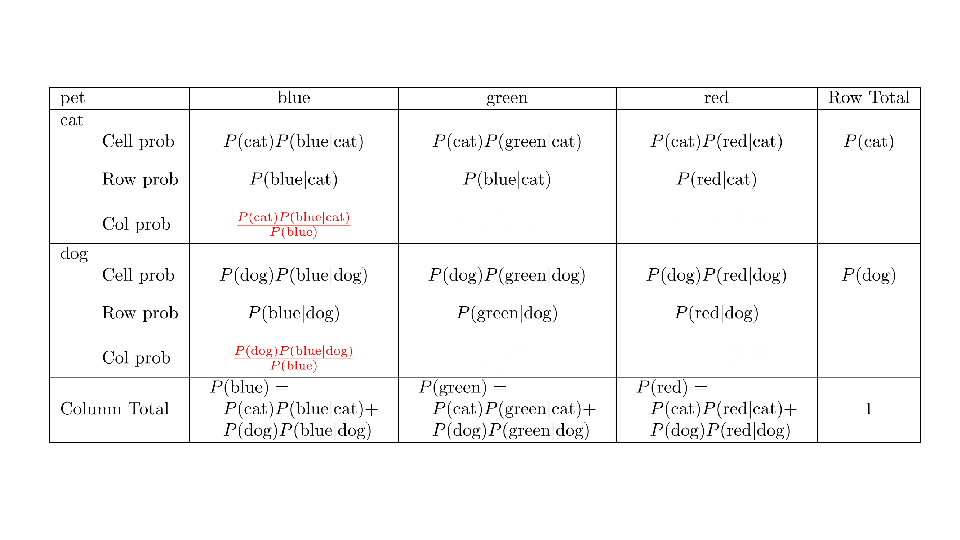
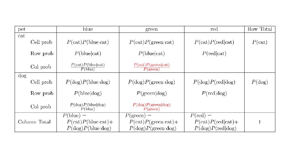
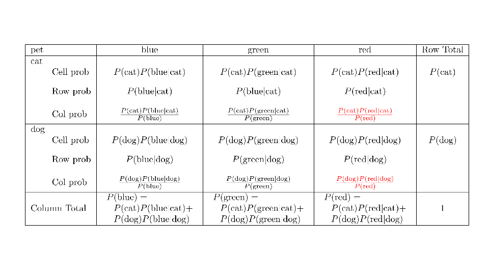
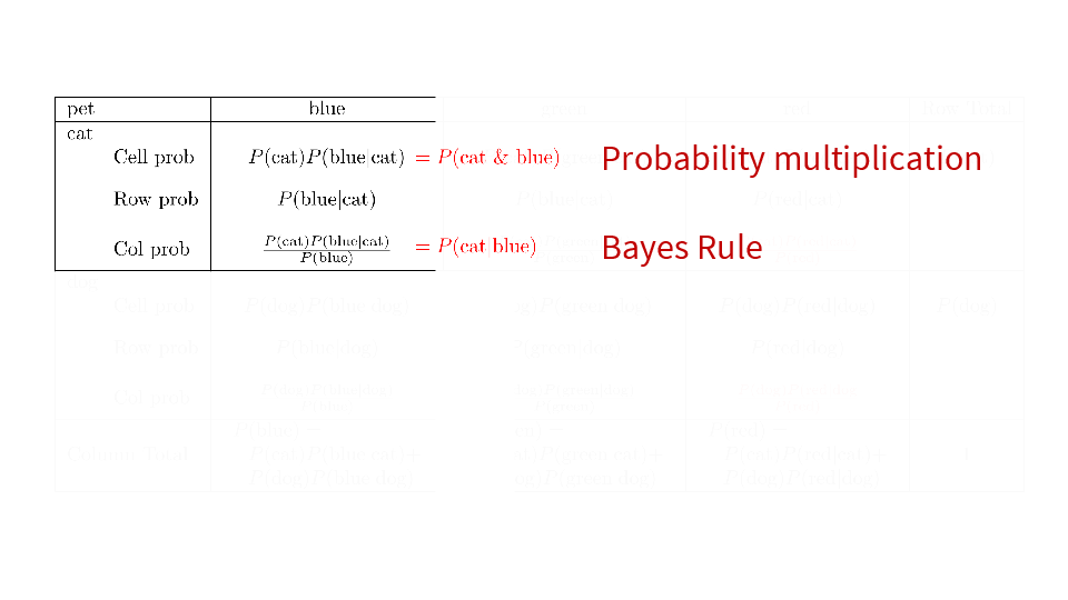
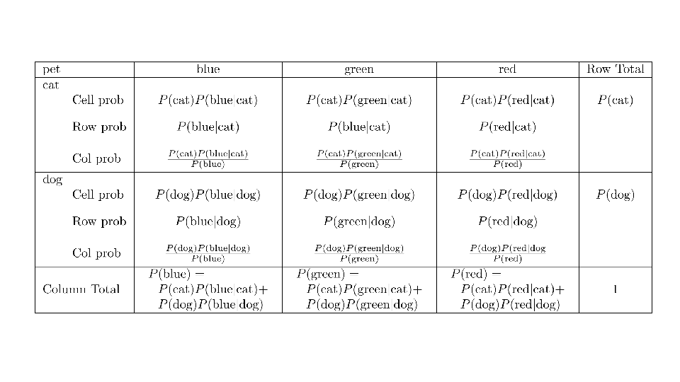
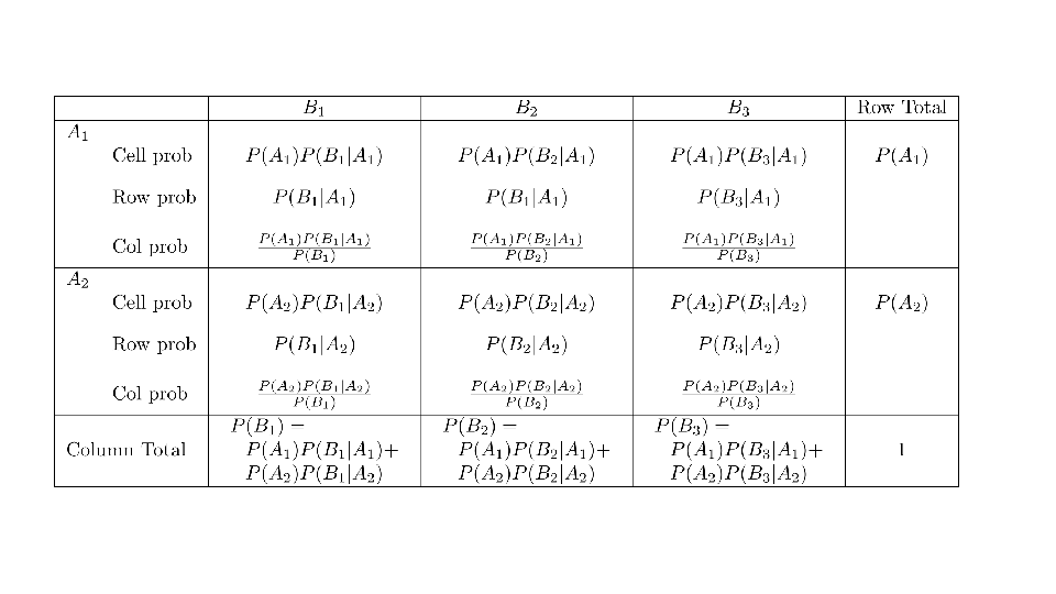
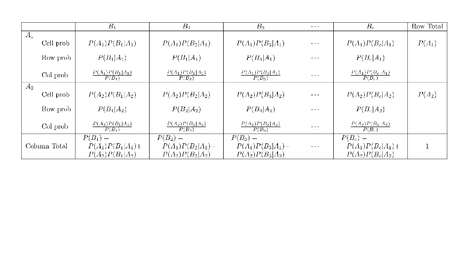
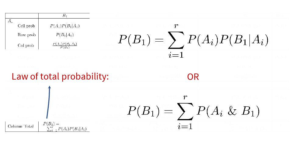
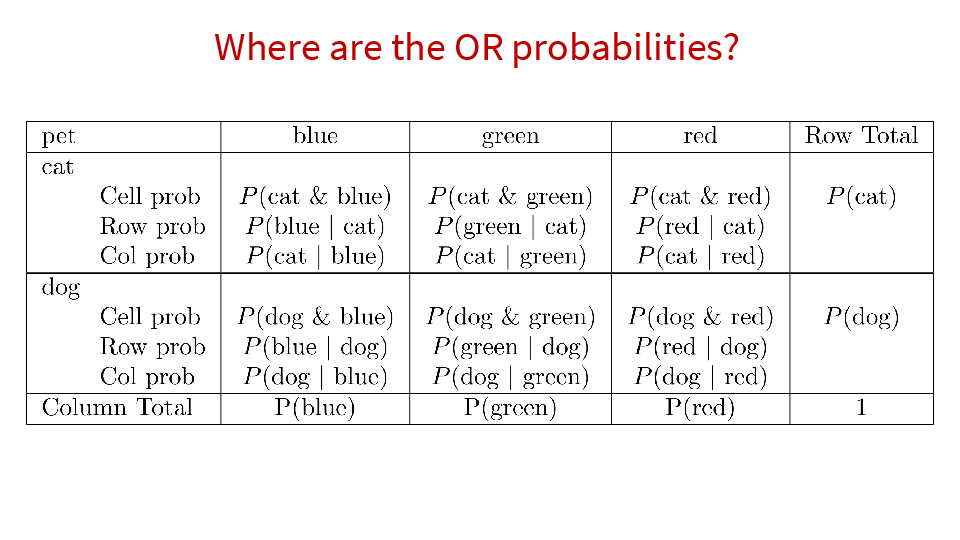
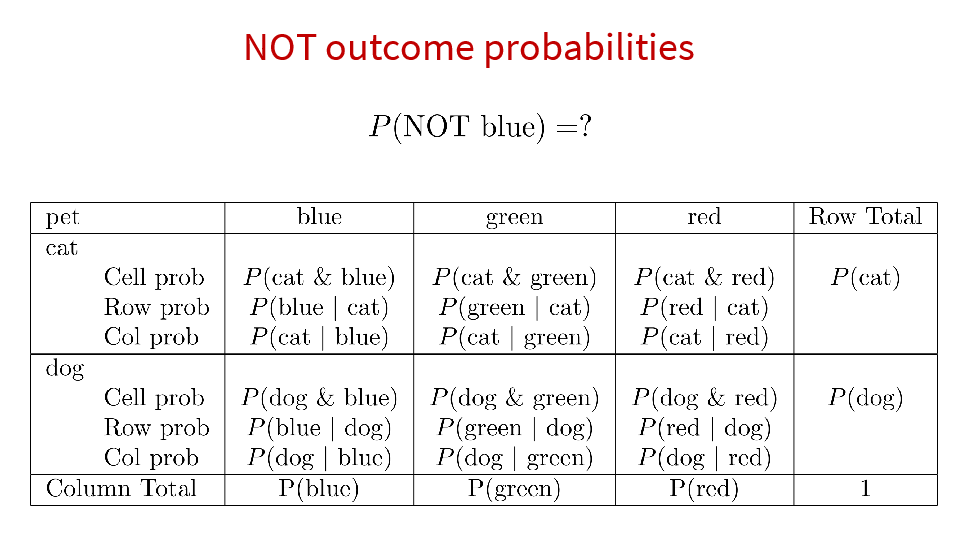
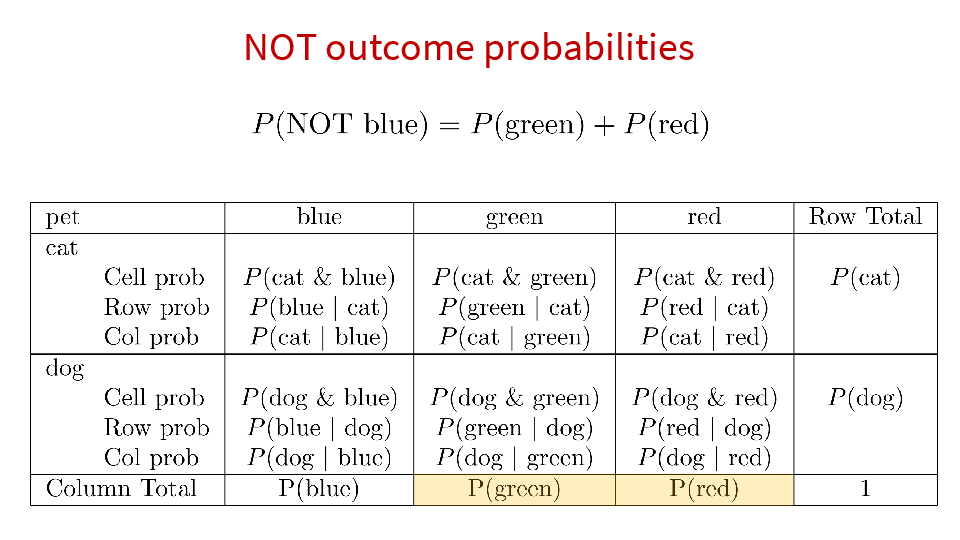
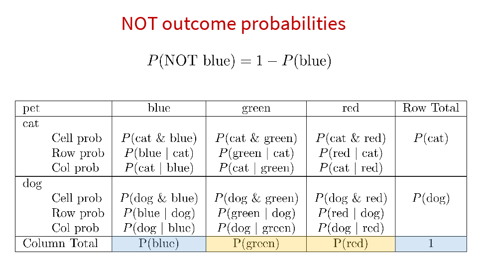
4.2 Cross tabs
When working with two outcomes, it is often helpful to organize the data into a cross table. In the table below, the counts of two outcomes—favorite color and pet preference—are tabulated. Favorite color has three options: blue, green, and red. Pet preference has two options: cat or dog. The cross table shows the counts of all possible joint outcomes; there are 6. Rather than listing the counts as a list, the counts are reported in a matrix, with pet preference along the rows and color preference along the columns.