10 Calculus

Calculus is an important area of mathematics widely applied in data science applications. In this class, we will use calculus for two important tasks:

Find the value of $x$ which maximizes (or minimizes) the function $f(x)$ using derivatives and roots.
Find the area under $f(x)$ between $a$ and $b$ using antiderivatives or integration.

10.1 Some derivative and anti-derivatives to know for this class

For this class, a basic understanding of the derivatives and anti-derivatives of polynomials, logs/exponentials, and sin/cos will be helpful.

Condition	Function $f(x)$	Derivative	Anti derivative
$\beta \neq -1$	$\alpha x^{\beta}$	$\alpha\beta x^{\beta-1}$	$\alpha \frac{x^{\beta+1}}{\beta + 1} + C$
	$\alpha x^{-1}$	$-\alpha x^{-2}$	$\alpha \log(x) + C$
	$\alpha \log(x)$	$\alpha x^{-1}$	Not needed for DS 2026
	$\alpha e^{\beta x}$	$\alpha\beta e^{\beta x}$	$\alpha \frac{e^{\beta x}}{\beta} + C$
	$\alpha \sin(\beta x)$	$\alpha\beta \cos(\beta x)$	$-\alpha \frac{\cos(\beta x)}{\beta} + C$
	$\alpha \cos(\beta x)$	$-\alpha\beta \sin(\beta x)$	$\alpha \frac{\sin(\beta x)}{\beta} + C$

The following sections are examples of how these calculus topics are used in data science applications. This is not a review of calculus; rather, it is a few examples to hopefully spark the memories of what you’ve learned before.

10.2 TASK: Maximize (or minimize) $f(x)$

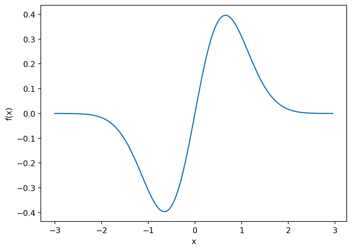
In the figure below, which value $x$ maximizes $f(x)$? Which value minimizes it? Because $f$ is a continuous function, we can use tools like the derivative to find the answers.

You’ll recall that the derivative of $f$ returns the instantaneous slope of $f$.

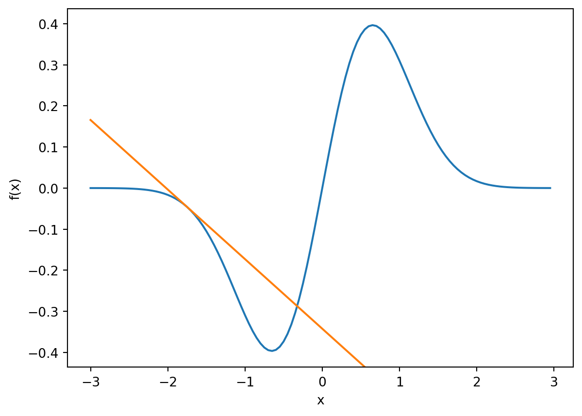
For a continous fuction, the local maximimums and minimums are going to occur at locations where the instantaneous slope is zero.

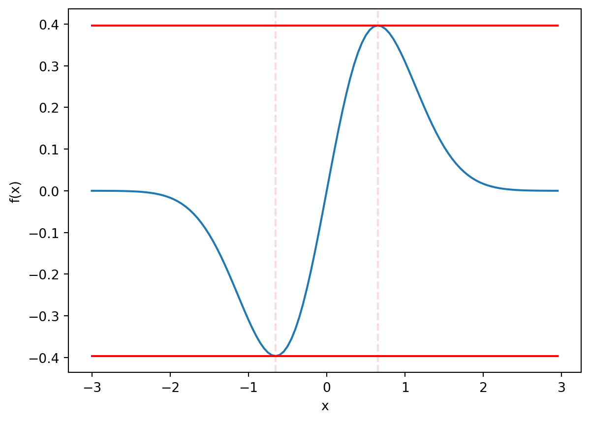
To find the local maximum and minimums of the function $f$, we can find the roots of its derivative.

There are lots of ways to denote the derivative:

\[ f' \quad\text{or}\quad f^{(1)} \quad\text{or}\quad \frac{d}{dx} f \quad\text{or}\quad \frac{df}{dx}. \]

10.2.1 Example: Maximum Likelihood

Consider 10 observations from the Rayleigh distribution.

x = np.array([3.12, 4.79, 0.05, 2.55, 1.69, 1.32, 1.93, 2.76, 3.02, 3.73])

The Rayleigh distribution with parameter $\theta$ has the following density:

\[ f(x;\theta) = \frac{x}{\theta}e^{-\frac{x^2}{2\theta}} \qquad x \geq 0,\quad \theta > 0 \]

If $\theta$ is unknown, one way to estimate it from the observed data $x$ using maximum likelihood. More details are provided in the estimation section, but the basic idea is to find the value of $\theta$ that maximizes the log likelihood function, which is

\[ \ell(\theta) = - n\log(\theta) - \frac{1}{2\theta}\sum_{i=1}^n x_i^2 \]

def l(theta, x):
    return -x.size * np.log(theta) - 1/2/theta * np.sum(x**2)

theta = np.arange(0.1,20,0.1)
y = l(theta,x)
plt.close()
plt.plot(theta,y)
plt.xlabel("θ")
plt.ylabel("log L(θ)")
plt.show()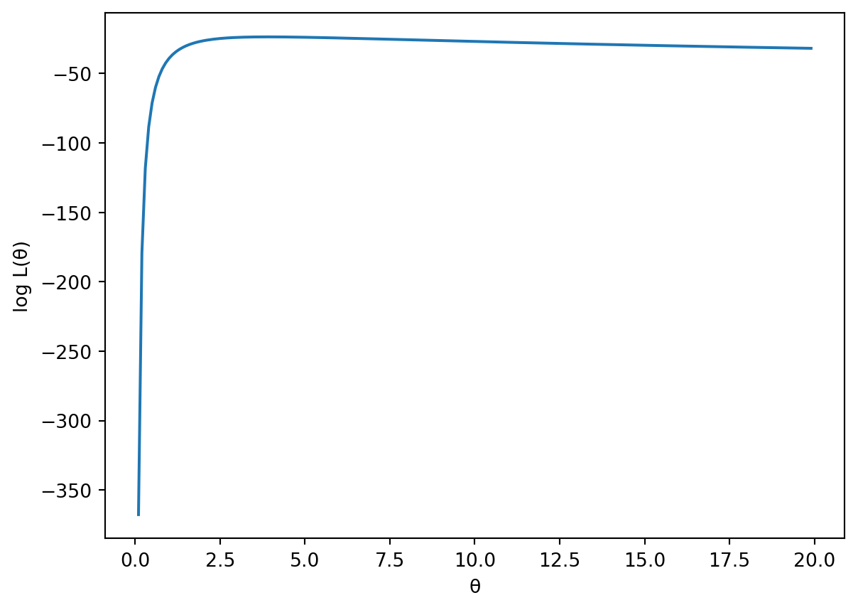

We can solve for $\theta$ by setting derivative of $\ell$ to zero.

\[ \begin{align*} \ell'(\theta) = -\frac{n}{\theta} + \frac{1}{2\theta^2}\sum_{i=1}^n x_i^2 &\overset{set}{=} 0\\ -n\theta + \frac{1}{2}\sum_{i=1}^n x_i^2&=0\\ \hat{\theta} &= \frac{1}{2n}\sum_{i=1}^n x_i^2 \end{align*} \]

theta_hat = np.sum(x**2)/2/x.size
f'{theta_hat:.3f}'

'3.908'

Based on the 10 observations, best guess is $\hat{\theta} = 3.908$ . Based on the picture of the likelihood, this value maximizes the likelihood. We could also verify this fact using the second derivative.

Let’s generate a few more observations so that we can visualize the distribution and compare it to the MLE estiamte. With 1000 draws, the histogram matches up nicely with the MLE density estimate. Likewise for the emperical CDF and the MLE CDF estimate.

np.random.seed(1)
x = 3*np.sqrt(-2*np.log(1-np.random.uniform(size=1000)))
plt.close()

fig, (plt1, plt2) = plt.subplots(1, 2)

plt1.hist(x, density=True, bins=30, label = "Histogram")
def f(x,theta):
    return x/theta * np.exp(-x**2/theta/2)
theta_hat = np.sum(x**2)/2/x.size
xx = np.arange(0,10,0.1)
plt1.plot(xx,f(xx,theta_hat), label = "MLE density estimate")
plt1.legend()

def F(x,theta):
    return 1 - np.exp(-x**2/theta/2)
from statsmodels.distributions.empirical_distribution import ECDF
p = ECDF(x)
plt2.plot(p.x, p.y, label = "ECDF")
plt2.plot(xx,F(xx, theta_hat), label = "MLE CDF estimate")
plt2.legend()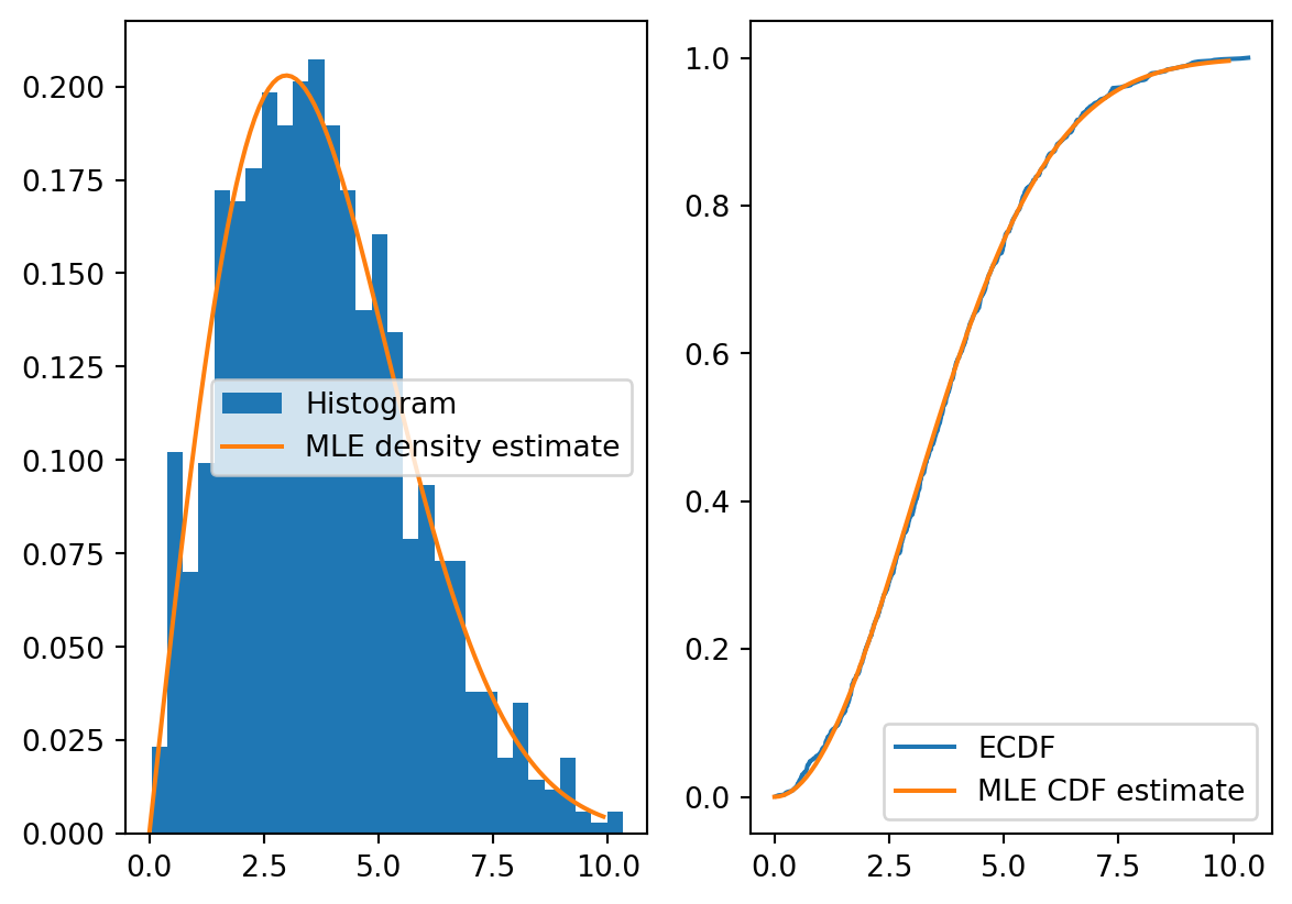

10.2.2 Example: Line fitting

np.random.seed(1)
x = np.random.normal(size = 10)
y = 2 - 0.3*x + np.random.normal(scale = 0.25, size = 10)
plt.close()
plt.scatter(x,y)
plt.xlabel("x")
plt.ylabel("y")
plt.show()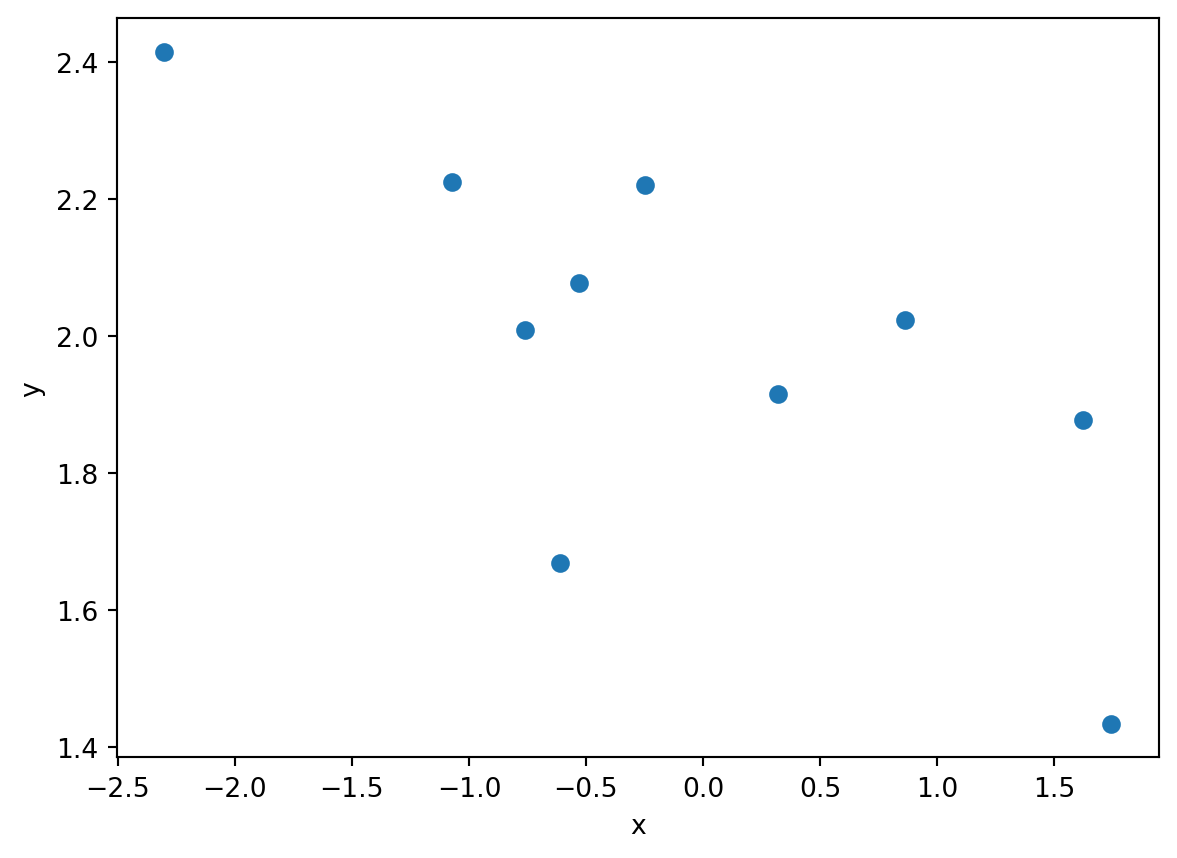

Given a set of points $(x_i, y_i)$, one might want to estimate the relationship between $x$ and the mean of $y$,

\[ E[y|x_i] = f(x_i) \]

If we assume a linear relationship, the relationship to be estimated is

\[ E[y|x_i] = \alpha + \beta x_i \]

where $\alpha$ and $\beta$ are unknown parameters. One method to estimate this relationship is select the values of $\alpha$ and $\beta$ which minimize the sum of squared errors,

\[ \begin{align*} \text{sum of squared errors:}\quad SSE &= \sum_{i=1}^n (\underbrace{y_i - \alpha - \beta x_i}_{\text{error } e_i})^2 \end{align*} \]

In this example, because there are two parameters, we want to find the value of $\alpha$ and $\beta$ that simultaneously minimizes the sum of squared errors. The figure below shows the SSE surface. Looking at the figure suggests that an $\alpha$ close to 2 and $\beta$ close slightly less than 0 is the minimum.

alphas = np.linspace(-5, 5, 100)
betas = np.linspace(-5, 5, 100)
A, B = np.meshgrid(alphas, betas)
sse = A*0
for i in range(100):
    for j in range(100):
        e = y - A[i,j] - B[i,j]*x
        sse[i,j] = sum(e**2)
plt.close()
plt.contourf(A, B, np.log(sse), levels = 20, cmap = "magma")
plt.colorbar()
plt.xlabel("α")
plt.ylabel("β")
plt.show()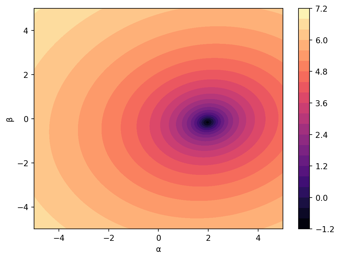

We can use the derivative to find the exact minimum sum of squared errors. In the next expression, we use the bar notation to denote a sample average, as in $\bar{z} = 1/n\sum_i z_i$.

\[ \begin{align*} 0 &\overset{set}{=} \frac{d\, SSE}{\partial \alpha} \\ &= \sum_{i=1}^n 2(y_i - \alpha - \beta x_i)(-1)\\ &= -2n(\bar{y} - \alpha - \beta \bar{x})\\ 0 &= \bar{y} - \alpha - \beta \bar{x} \end{align*} \]

Now the partial derivative with respect to $\beta$.

\[ \begin{align*} 0 &\overset{set}{=} \frac{d\, SSE}{\partial \beta} \\ &= \sum_{i=1}^n 2(y_i - \alpha - \beta x_i)(-x_i)\\ &= -2n(\bar{yx} - \alpha\bar{x} - \beta \bar{x^2})\\ 0 &= \bar{yx} - \alpha\bar{x} - \beta \bar{x^2} \end{align*} \]

We have two equations and two unknowns. Using substitution, we plug $\alpha = \bar{y} - \beta\bar{x}$ into the second equation and solve for $\beta$:

\[ \begin{align*} 0 &= \bar{yx} - \alpha\bar{x} - \beta \bar{x^2} \\ &= \bar{yx} - (\bar{y} - \beta\bar{x})\bar{x} - \beta \bar{x^2} \\ &= \bar{yx} - \bar{y}\bar{x} + \beta\bar{x}^2 - \beta \bar{x^2} \\ &= \bar{yx} - \bar{y}\bar{x} + \beta(\bar{x}^2 - \bar{x^2}) \\ \frac{\bar{y}\bar{x} - \bar{yx}}{\bar{x}^2 - \bar{x^2}} &= \hat{\beta} \end{align*} \]

Plugging $\hat{\beta}$ back into the first equation we solve for $\alpha$:

\[ \begin{align*} \hat{\alpha} &= \bar{y} - \hat{\beta}\bar{x}\\ &= \bar{y} - \frac{\bar{y}\bar{x} - \bar{yx}}{\bar{x}^2 - \bar{x^2}}\bar{x}\\ \end{align*} \]

Plugging in the data, we get the straight line relationship that minimizes the sum of squared errors.

plt.close()
plt.scatter(x,y)
plt.xlabel("x")
plt.ylabel("y")
ybar = y.mean()
yxbar = (y*x).mean()
xxbar = (x*x).mean()
xbar = x.mean()
beta_hat = (xbar*ybar - yxbar)/(xbar**2 - xxbar)
alpha_hat = ybar - beta_hat*xbar

xx = np.arange(min(x), max(x),0.01)
yy = alpha_hat + beta_hat*xx
plt.plot(xx,yy, label = "Min SSE line")
plt.legend()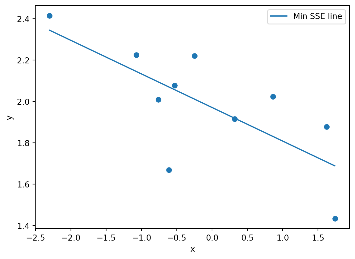

10.3 Area under $f(x)$

The density function of a continuous random variable encodes probabilities as areas under the curve. If $f$ is the density function of the random variable $X$, then

\[ P(a \leq X \leq b) = \text{area under $f$ between $a$ and $b$} \]

import scipy.stats as st

x = np.linspace(0, 100, 1000)
pdf = st.norm.pdf(x,loc = 70, scale=9)
plt.close()
plt.plot(x, pdf, linewidth=2)
x_fill = x[(x >= 70) & (x <= 75)]
pdf_fill = st.norm.pdf(x_fill,loc = 70, scale=9)
plt.fill_between(x_fill, pdf_fill, alpha=0.3, label='Shaded region')
plt.xlabel('x')
plt.ylabel('Density')
plt.xticks([70,75], labels=['a','b'])
plt.show()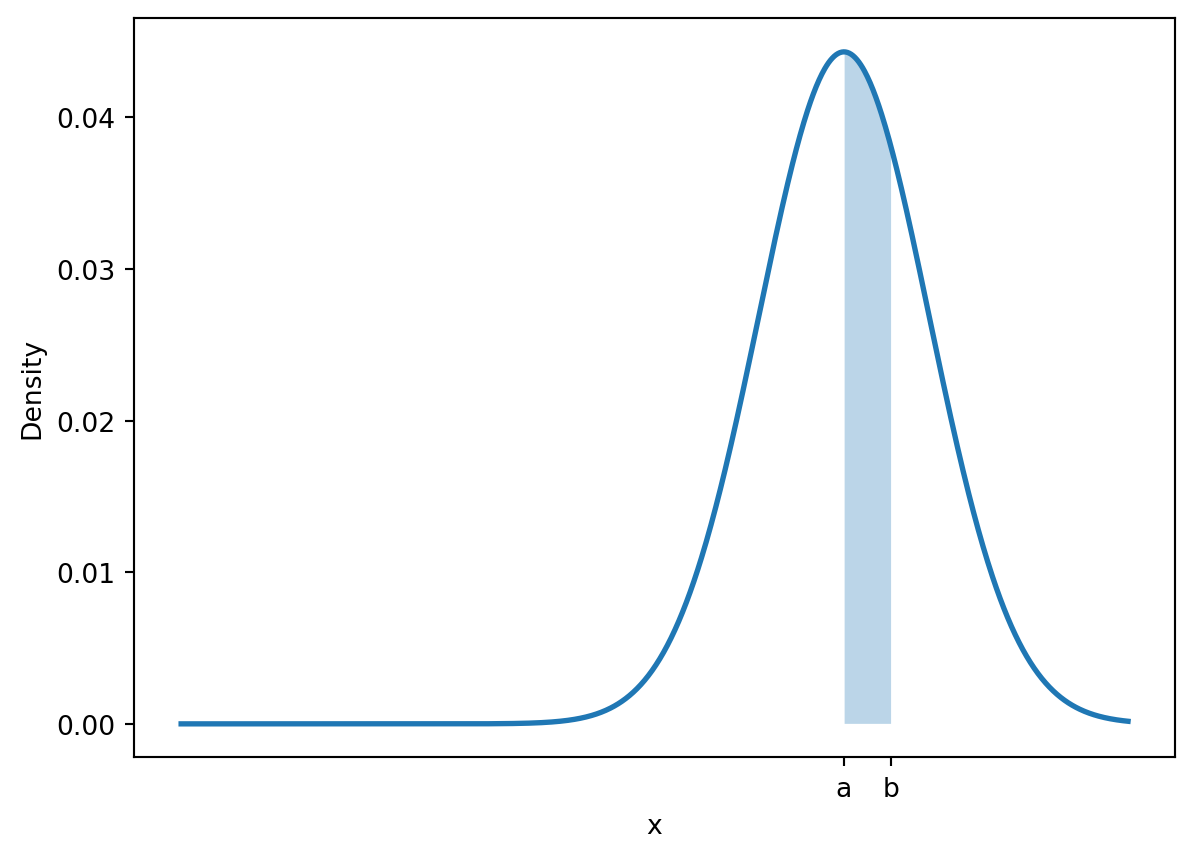

Because integrals calculate the area under curves, integrals are used widely in probability calculations.

10.3.1 Example

Consider the triangle that is formed by randomly selecting 3 points on the unit circle.

fig, plt1 = plt.subplots(subplot_kw={'projection': 'polar'})
theta = np.linspace(0, 2*np.pi, 100)
r = 0*theta + 1
plt1.plot(theta,r)
plt1.axis('off')
np.random.seed(2)
ts = np.random.uniform(0,2*np.pi,size=3)
ts = np.append(ts, ts[0])
rs = 1 + 0*ts
plt1.scatter(ts, rs)
plt1.plot(ts,rs)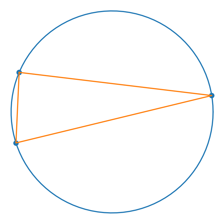

The density function of the area of such triangles is an interesting shape. In the figure below, we approximated the density with a scaled beta distribution.

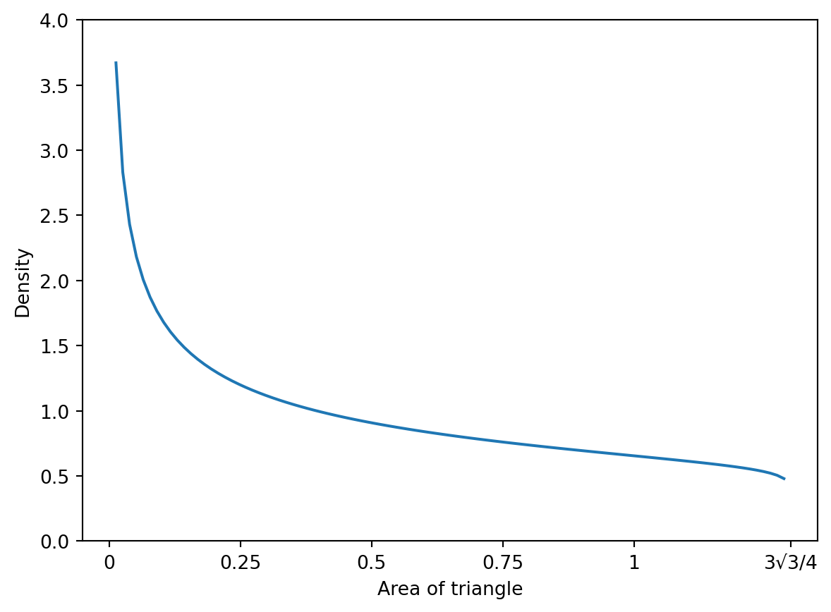
If we wanted to find the probability that a random triangle has area less than 1, we could integrate the density or use the cumulative density function (CDF) if it is available. The CDF is the integral of the density function. The lower bound of the integral is often written with negative infinity, but that is shorthand for the minimum value of the random variable. In our triangle example, the minimum value is 0.

\[ CDF(x) = \int_{-\infty}^x f(t)\,dt \]

In Python, the integral of the beta distribution is included in the scipy.stats package.

import scipy.stats as st
st.beta.cdf(1/scale, a_fit, b_fit)

np.float64(0.8657492986142342)

10.3.2 Example

When a problem requires an integral for a distribution not in python, we can use calculus. Consider this odd distribution.

\[ f(x) = \frac{1}{4\pi}(\sin(x) + 1) \qquad -2\pi \leq x \leq 2\pi \]

def f(x):
    return 1/np.pi/4*(np.sin(x)+1)
x = np.arange(-2*np.pi, 2*np.pi,0.01)
y = f(x)
plt.close()
plt.plot(x,y)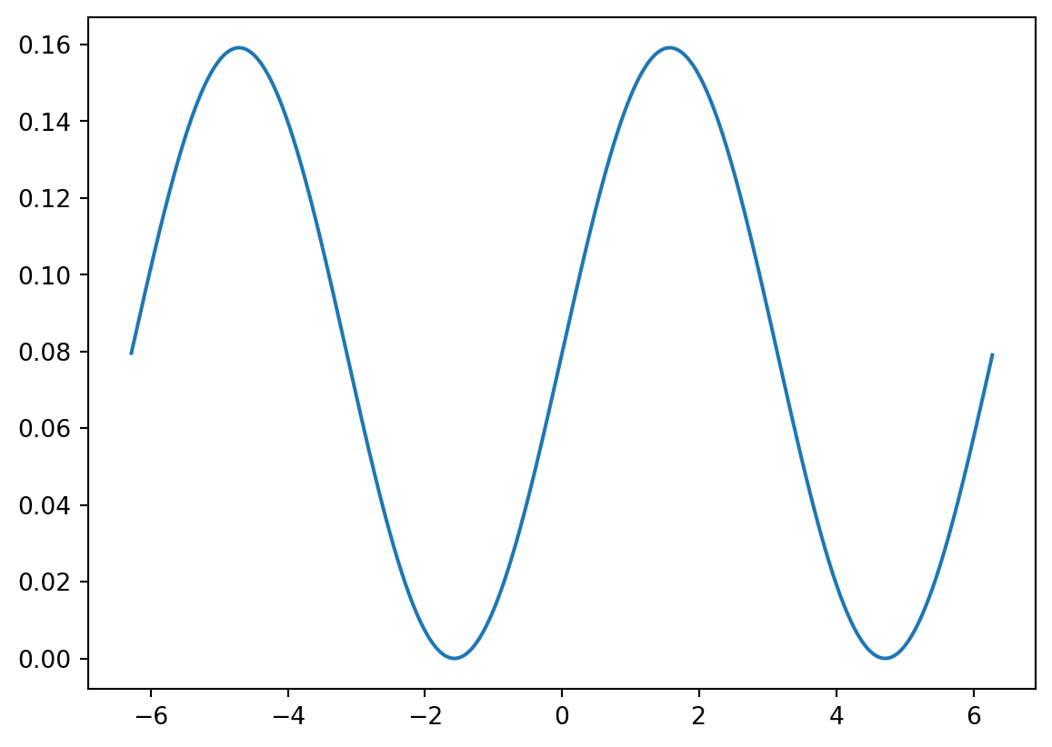

We can find the CDF function.

\[ \begin{align*} F(x) &= \int_{-2\pi}^x \frac{1}{4\pi}(\sin(t) + 1)\,dt\\ &= \left.\frac{1}{4\pi}[-\cos(t) + t] \right|^x_{-2\pi}\\ &= \frac{1}{4\pi}[-\cos(x) + x + \cos(-2\pi)-(-2\pi)] \\ &= \frac{1}{4\pi}[-\cos(x) + x + 1+2\pi]\\ &= \frac{1}{4\pi}[1+2\pi + x -\cos(x)] \end{align*} \]

def F(x):
    return 1/4/np.pi*(1+2*np.pi + x - np.cos(x))
Y = F(x)
plt.close()
plt.plot(x,Y)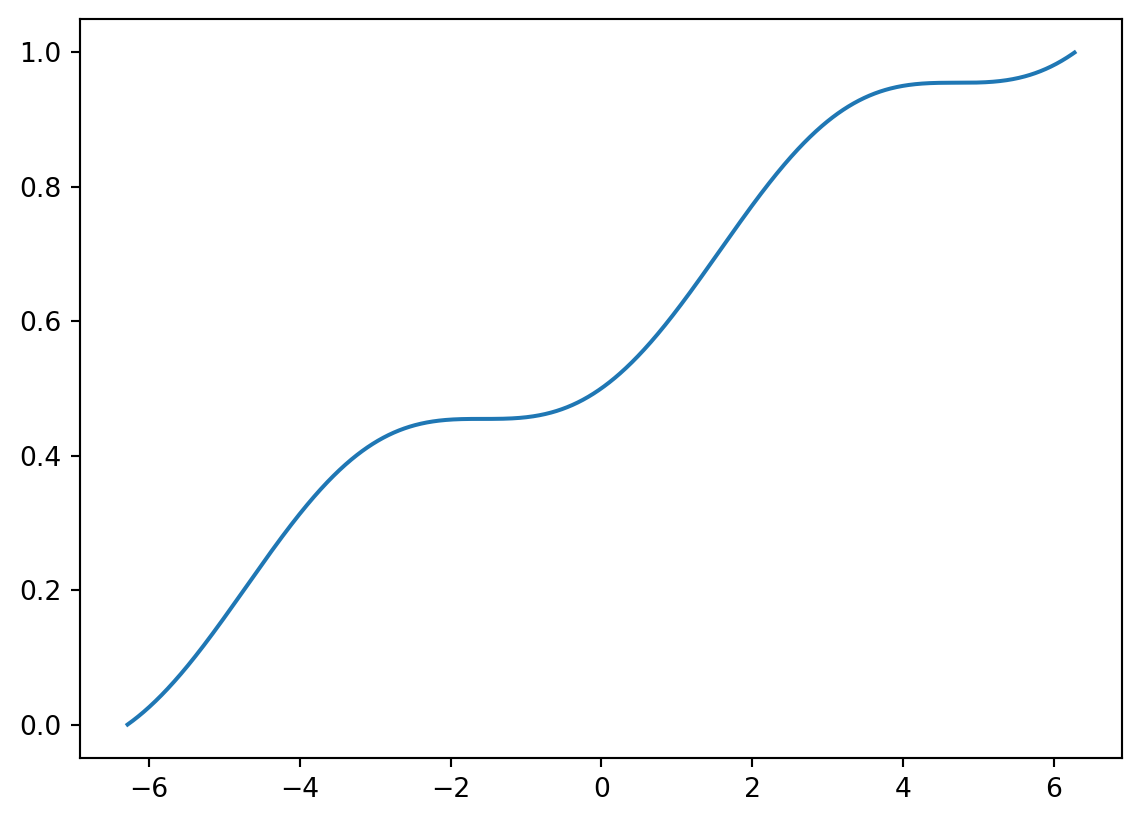

It is not a typical distribution, but you’ll notice that all the rules for a CDF satisfied. We can use it to calculate probabilities:

\[ P(-4 \leq X \leq -2) = F(-2) - F(-4) = \frac{1}{4\pi}[1+2\pi + -2 -\cos(-2)] - \frac{1}{4\pi}[1+2\pi + -4 -\cos(-4)] \approx 0.14 \]

F(-2) - F(-4)

np.float64(0.1402555494956974)

Condition	Function \(f(x)\)	Derivative	Anti derivative
\(\beta \neq -1\)	\(\alpha x^{\beta}\)	\(\alpha\beta x^{\beta-1}\)	\(\alpha \frac{x^{\beta+1}}{\beta + 1} + C\)
	\(\alpha x^{-1}\)	\(-\alpha x^{-2}\)	\(\alpha \log(x) + C\)
	\(\alpha \log(x)\)	\(\alpha x^{-1}\)	Not needed for DS 2026
	\(\alpha e^{\beta x}\)	\(\alpha\beta e^{\beta x}\)	\(\alpha \frac{e^{\beta x}}{\beta} + C\)
	\(\alpha \sin(\beta x)\)	\(\alpha\beta \cos(\beta x)\)	\(-\alpha \frac{\cos(\beta x)}{\beta} + C\)
	\(\alpha \cos(\beta x)\)	\(-\alpha\beta \sin(\beta x)\)	\(\alpha \frac{\sin(\beta x)}{\beta} + C\)