9 Continuous Random Variables
A continuous random variable takes values on an interval of the real line \(R\).
Examples of continuous random variables include:
The height \(H\) of a student: in cm, \(0\le H \le 300\).
The temperature \(T\) of a room: in Celsius, \(-273.15 \le T \le \infty\).
The time \(T\) it takes for a light bulb to burn out: in seconds, \(0 \le T \le \infty\).
9.1 Cumulative Distribution Function
The distribution function, also known as the cumulative distribution function (CDF), of a random variable \(X\) provides a comprehensive description of its probability distribution. It is defined as follows:
The distribution function \(F\) of the random variable \(X\) is the function
\[F(x) = P(X\le x)= P(\omega : X(\omega) \le x), \qquad x \in R\]
In simpler terms, the CDF, denoted as \(F(x)\) or \(F_X(x)\) to emphasize the random variable, gives the probability that the random variable \(X\) takes on a value less than or equal to a given value \(x\).
9.1.1 Examples:
- Uniform Distribution, \(U(a,b)\)
\[ F(x) = \begin{cases} 0 & \; & x\le a \\ \frac{x-a}{b-a} & \; & a<x<b \\ 1 & \; & b\le x \end{cases} \]
- Exponential Distribution, \(Exp(\lambda)\)
\[ F(x) = \begin{cases} 0 & \; & x \le 0 \\ \\ 1- e^{-\lambda x} & \; & 0 < x \; \lambda > 0 \end{cases} \]
- Normal Distribution, \(N(\mu,\sigma)\)
\[ F(x) = \frac{1}{\sqrt{2\pi\sigma^2}}\int_{-\infty}^{x} e^{\frac{(u-\mu)^2}{2\sigma^2}}du \] We do not know how to solve that integral using simple functions (polynomials, trig function, exp, logs, algebraic functions, etc.), so we have to keep as it is. Maybe this is a suggestion to write all \(F(x)\) as integrals, and use the integrated function (\(\frac{1}{\sqrt{2\pi}}e^{\frac{u^2}{2}}\)) instead?
- Binomial distribution, Binomial\((n,p)\)
9.1.2 Properties of the Cumulative Distribution Function
The CDF possesses several key properties:
Boundedness: \(0 \le F(x) \le 1\) for all \(x\).
Non-decreasing: \(P(x < X \le y) = F(y) - F(x) \ge 0\), for all \(x \le y\).
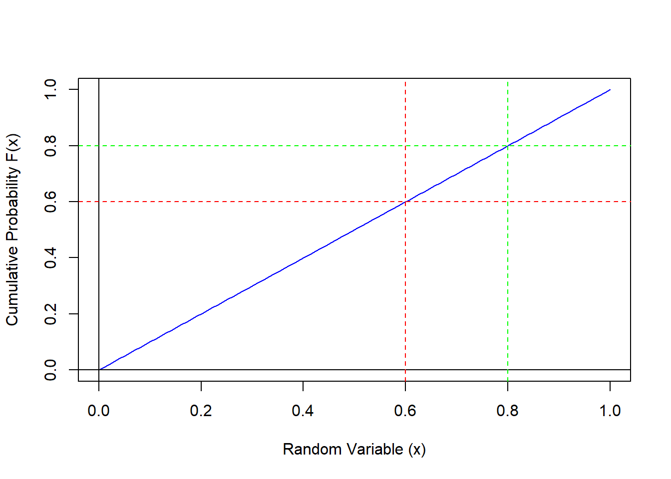
- Graphical Example for X with Uniform(0, 1)
\[ P(.6 < X < .8) = F(.8) - F(.6) = .8 - .6 = .2 \]
Right-continuous: If \(h>0\), then \[\lim_{h \to 0} F(x+h) = F(x).\]
Limits at Infinity: \[\lim_{x \to \infty} F(x) = 1 \text{ and } \lim_{x \to -\infty} F(x) = 0.\]
Any function satisfying these properties can be the distribution function of some random variable.
9.1.3 Probability of a Single Point
An important consequence of the continuity of the CDF is the following result:
If \(X\) has a continuous distribution function \(F\), then \[ P(X = x) = 0 \qquad \text{for all} \quad x \]
Check:
We can express the probability of \(X\) taking a specific value \(x\) as a limit of probabilities over shrinking intervals:
\[P(X = x) = \lim_{n \to \infty} P \left( x - \frac{1}{n} < X \le x \right)\]
Using the properties of the CDF from Theorem (6), this can be rewritten as:
\[= \lim_{n \to \infty} \left( F(x) - F \left( x - \frac{1}{n} \right) \right)\]
Since \(F\) is continuous, the limit as \(n\) approaches infinity becomes:
\[ = F(x) - F(x) = 0.\]
This result highlights a crucial distinction between discrete and continuous random variables. While for discrete variables the probability of individual points can be non-zero, for continuous variables, it is always zero.
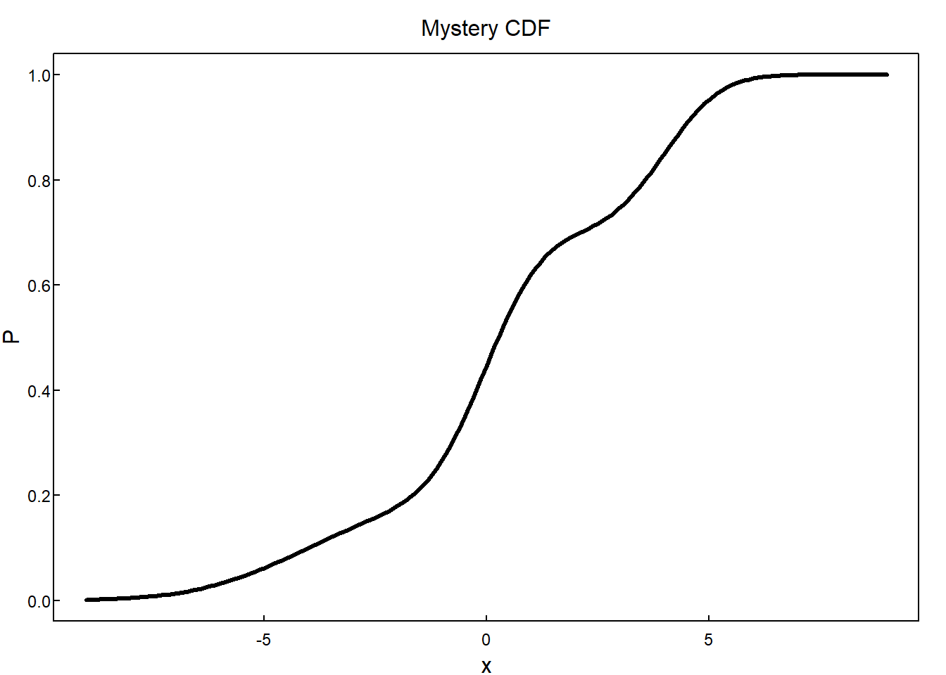
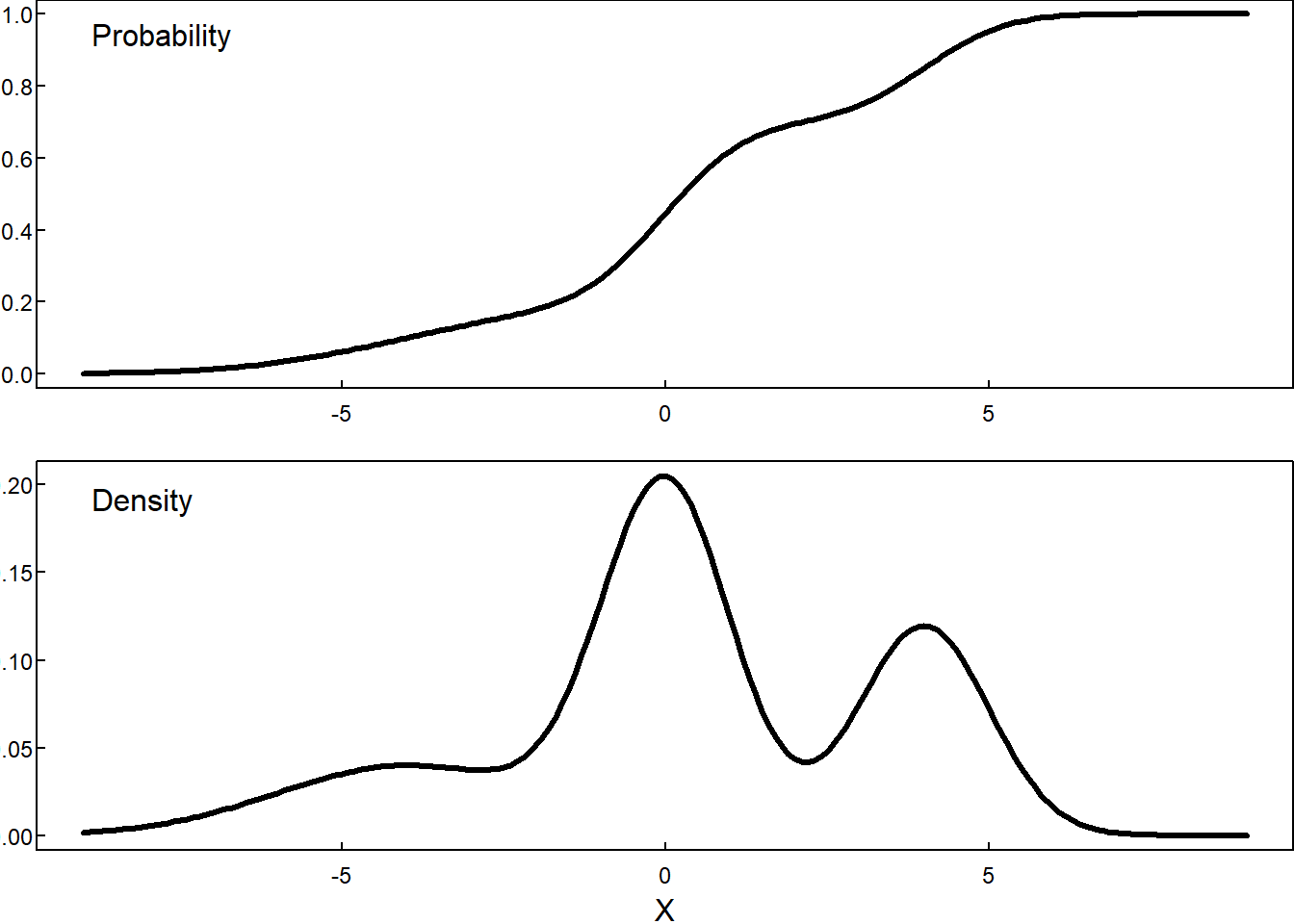
9.1.4 Mystery CDF
Questions:
- What can we learn from the CDF?
- What is going on in the regions that are flatter?
- What is going on in the regions that are steeper?
- Where is the median?
- Where is the 25th percentile? 75th percentile?
Answers:
- We can identify quantiles and outcomes.
- Values in flatter intervals are less likely to occur than values in steeper intervals. The derivative (a measure of flatness/steepness) of the CDF (if it exists) is the relative likelihood, also called the probability density function.
- See previous answer.
- To find the median, draw the horizonal line \(y = 0.5\). The x value where that line intersects the CDF is the median.
- Use the same procedure as the previous answer with \(y=0.25\) and \(y=0.75\).
9.2 Density Function
The density function provides a more intuitive way to understand the distribution of a continuous random variable. It is linked to the CDF through differentiation:
Definition: Let \(X\) have distribution function (CDF) \(F\). If the derivative
\[ \frac{dF}{dx} = F'(x) \]
exists at all but a finite number of points, and the function \(f\) defined by
\[ f(x) = \begin{cases} F'(x), & \text{where } F'(x) \text{ exists} \\ 0, & \text{elsewhere} \end{cases} \]
satisfies
\[ F(x) = \int_{-\infty}^x f(v) dv, \]
then \(X\) is said to be a continuous random variable with density \(f(x)\).
The density function, \(f(x)\), represents the probability density at a given point \(x\). It’s important to remember that \(f(x)\) itself is not a probability but a measure of how dense the probability is around \(x\).
9.2.1 Density functions cannot be negative
Because (a) probability functions are non-decreasing and (b) the density function is the derivative of the probability function, the density function can never be negative,
\[ f(x) \geq 0 \quad \textrm{for all } x \]
9.2.2 Density functions encode probability as area under the curve
If \(X\) has density \(f(x)\), then for a set \(C \subseteq R\), the probability of \(X\) falling within \(C\) is obtained by integrating the density function over that set:
\[P(X \in C) = \int_C f(x) dx.\]
For example, \(P(X<1) = F(1)\) is the area under the density curve to the left of \(x = 1\).
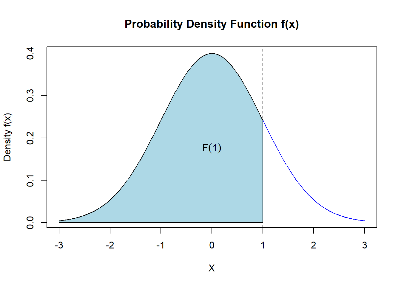
\[ F(1) = \int_{-\infty}^1 f(x) dx \]
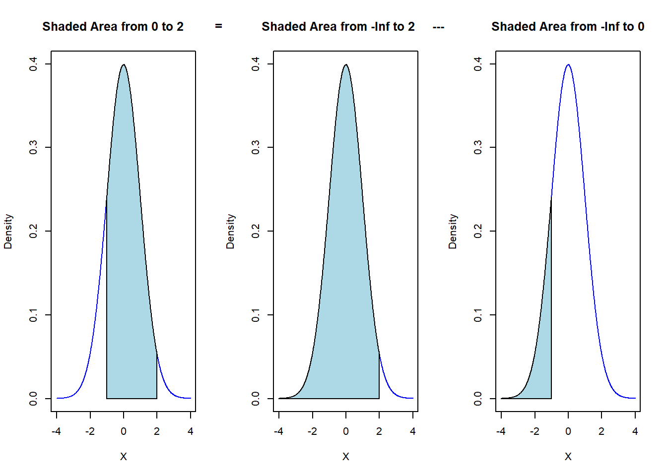
Likewise, the probability the outcome occurs between 0 and 2 is the area under the density curve from 0 to 2.
\[ P(0<X<2) = \int_{0}^2 f(x) dx = \int_{-\infty}^2 f(x) dx - \int_{-\infty}^1 f(x) dx \]
9.2.3 The area under the density curve must be 1
Recall that the probability function is or approaches 1 as \(x\) goes to infinity.
\[ \lim_{x\to\infty} P(X \leq x) = \lim_{x\to\infty} F(x) = 1 \]
As a consequence, the area under the density curve must be 1.
\[ \int_{-\infty}^{\infty} f(x) dx = 1 \]
This is a helpful property when a distribution is known up to a constant. For example, we might now that the density of a random variable has the following shape, but \(c\) is unknown.
Because the area under the curve must be 1, we can find c. In this case, we can use geometry to solve for \(c\). The area of the triangle is \(2c\). Because \(2c = 1\),
\[ c = \frac{1}{2} \]
In other cases, we will need to use calculus. For example, suppose the density of a random variable is
\[ f(x) = c*x^2\quad 0 \leq x \leq 1. \]
Then
\[ \begin{array}{rl} 1 &= \int_0^1 cx^2\, dx \\ &= c\int_0^1 x^2\, dx \\ &= c \left(\left.\frac{x^3}{3}\right|_0^1\right) \\ &= c\frac{1}{3} \\ 3 &= c \end{array} \]
9.3 Distributions
In the sections that follow, we describe some of the most commonly used distributions for continuous outcomes.
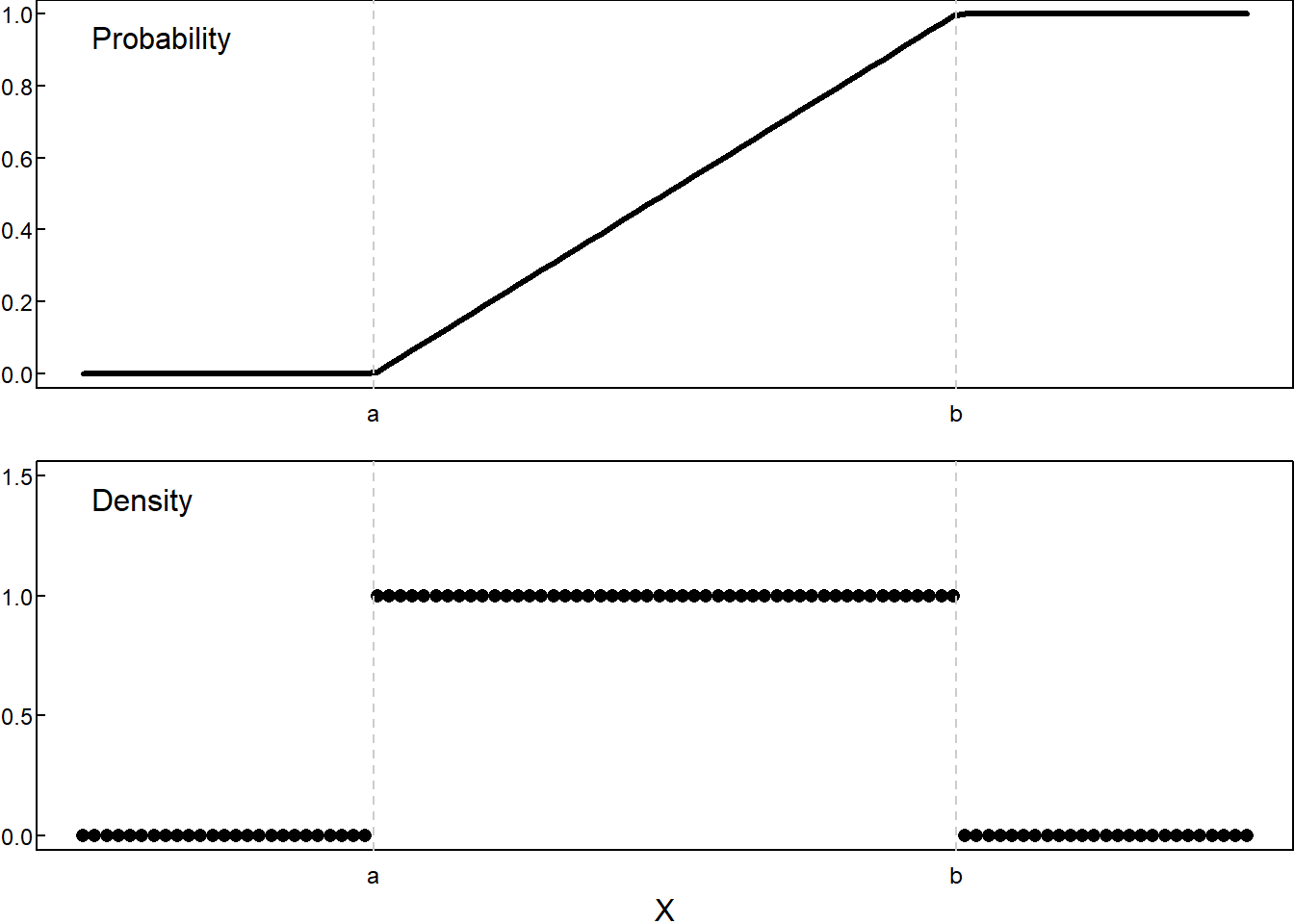
9.3.1 Uniform
\[ F(x) = \begin{cases} 0 & \; & x< a \\ \frac{x-a}{b-a} & \; & a\le x \le b \\ 1 & \; & b < x \end{cases} \qquad \qquad f(x) = \begin{cases} 0 & x < a\\ \frac{1}{b-a}, & a \le x \le b \\ 0, & b < x \end{cases} \]

Two parameters:
- \(a\), left end point
- \(b\), right end point
All values between \(a\) and \(b\) are equally likely to occur.
Applications
- Generation of random variables from other distributions. (How might one generate a Bernoulli random variable from a uniform random variable?)
- Maximum uncertainty models
Code
from scipy.stats import uniform
# Define distribution: Uniform(a, b) on interval [a, b]
# IMPORTANT: scipy uses loc=a and scale=(b-a), NOT loc=a and scale=b
# For Uniform[2, 5]:
dist = uniform(loc=2, scale=3) # loc=lower bound, scale=width
# Alternatively, define your bounds and compute:
a, b = 2, 5
dist = uniform(loc=a, scale=b-a)
# PDF at a point
pdf_value = dist.pdf(3.5) # Returns 1/(b-a) if a ≤ x ≤ b, else 0
# CDF at a point P(X ≤ x)
cdf_value = dist.cdf(4)
# Survival function P(X > x)
sf_value = dist.sf(4)
# Inverse CDF (percentiles)
median = dist.ppf(0.50) # Returns (a+b)/2
percentile_25 = dist.ppf(0.25)
# Probability in an interval P(c < X < d)
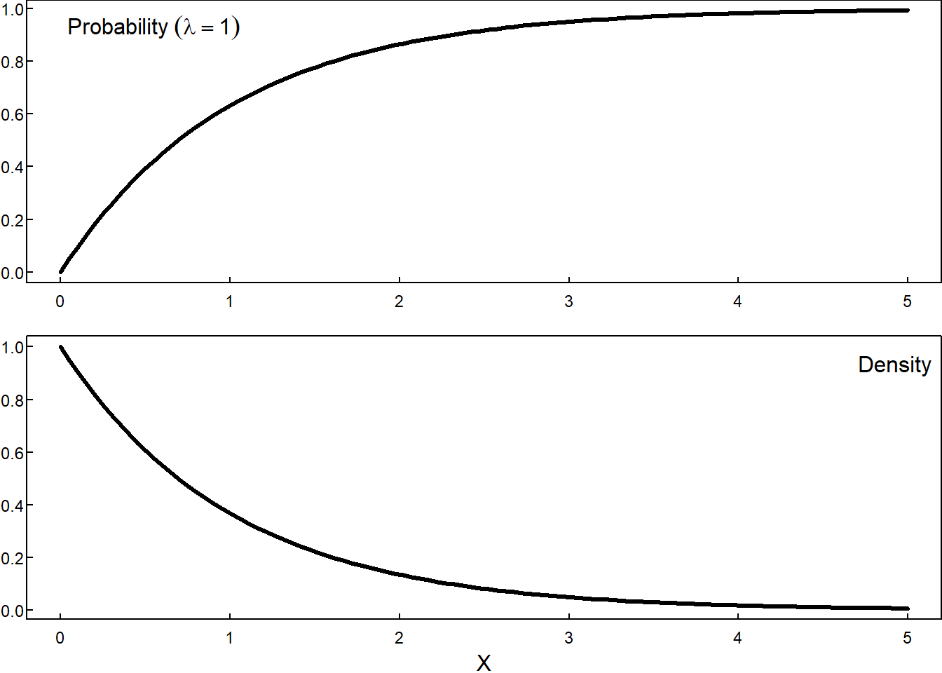
prob = dist.cdf(4.5) - dist.cdf(3.0)9.3.2 Exponential
The exponential random variable is frequently used to model the time until an event occurs, such as the time until a machine breaks down or the time between customer arrivals. Its density function is defined as:
\[ F(x) = \begin{cases} 0 & \; & x < 0 \\ \\ 1- e^{-\lambda x} & \; & 0 \le x \end{cases} \qquad \qquad f(x) = \begin{cases} 0, & x < 0\\ \\ \lambda e^{-\lambda x} & 0 \le x \end{cases} \]
where \(\lambda > 0\) is the rate parameter.
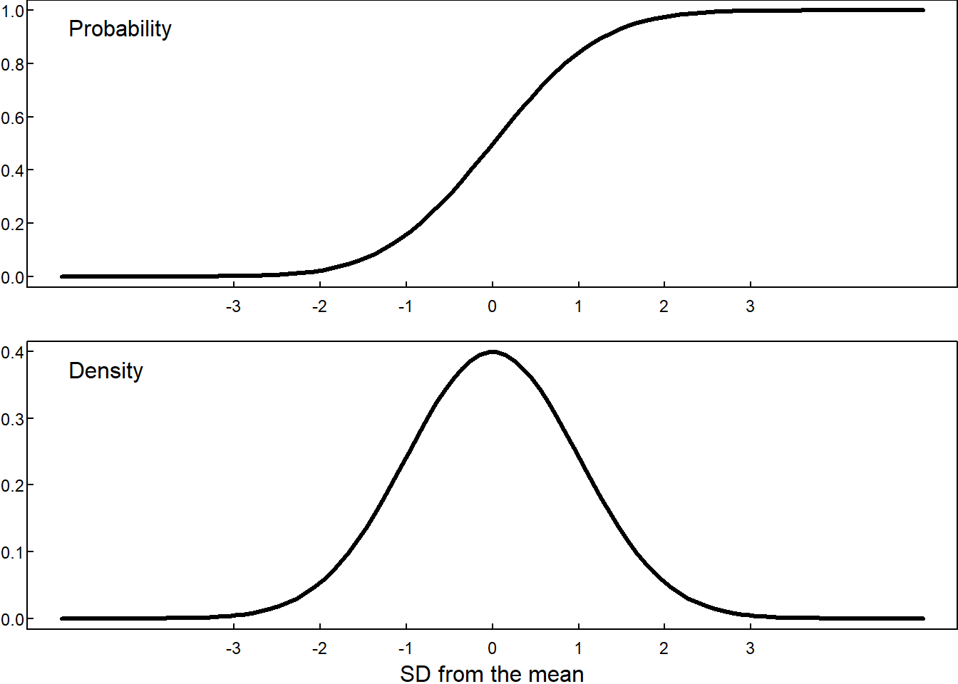
9.3.3 Normal
The normal random variable, also known as the Gaussian random variable, is ubiquitous in statistics due to its central role in the central limit theorem. Its density function has the characteristic bell shape
\[ F(x) = \frac{1}{\sqrt{2\pi \sigma^2}} \int_{-\infty}^x \exp \left( -\frac{(t - \mu)^2}{2\sigma^2} \right) dt, \qquad \qquad f(x) = \frac{1}{\sqrt{2\pi \sigma^2}} \exp \left( -\frac{(x - \mu)^2}{2\sigma^2} \right) \]
where \(\mu\) is the mean and \(\sigma^2\) is the variance.
Code
from scipy.stats import norm

dist = norm(loc=70, scale=3)

# PDF at a point
dist.pdf(72)
norm.pdf(72, loc=70, scale=3)

# CDF
cdf_value = dist.cdf(72)
norm.cdf(72, loc=70, scale=3)

# Probability in an interval P(a < X < b)
prob = dist.cdf(74) - dist.cdf(68)

# Inverse CDF (percentiles)
dist.ppf(0.25)
9.3.4 Gamma
The gamma random variable is a generalization of the exponential random variable and can model a wider range of phenomena. Its density function is given by:
\[ f(x) = \frac{c \lambda^\alpha x^{\alpha - 1} e^{-\lambda x}}{\Gamma(\alpha)}, \]
where \(\alpha > 0\) is the shape parameter, \(\lambda > 0\) is the rate parameter, and \(\Gamma(\alpha)\) is the gamma function.
Code
from scipy.stats import gamma

# Option 1: Using shape and rate
# Gamma(shape=α, rate=β)
# scipy uses scale = 1/rate
dist = gamma(a=3, scale=1/0.5)  # shape=3, rate=0.5

# Option 2: Using shape and scale
# Gamma(shape=α, scale=θ)
dist = gamma(a=2, scale=3)  # shape=2, scale=3

# PDF at a point
dist.pdf(10)

# CDF
dist.cdf(10)

# Inverse CDF
dist.ppf(0.50)
dist.ppf(0.75)
9.3.5 Beta
The beta random variable can model proportions and percentages, for instance the proportion of students left-handed at UVA.
\[ \frac{\Gamma(\alpha + \beta)}{\Gamma(\alpha)\Gamma(\beta)} t^{\alpha-1}(1-t)^{\beta-1} \]
where \(0 < t < 1\), and \(\alpha\) and \(\beta\) are parameters of the distribution.
[With \(\alpha=\beta=1\) we get the Uniform distribution U(0,1)]
Code
from scipy.stats import beta

# Define distribution: Beta(α, β)
dist = beta(a=3, b=7)

# PDF at a point
dist.pdf(0.25)
beta.pdf(0.25,a=3,b=7)

# CDF at a point (P(X ≤ x))
dist.cdf(0.40)
beta.cdf(0.4,a=3,b=7)

# Inverse CDF (quantile/percentile)
dist.ppf(0.50)
beta.ppf(0.50, a=3,b=7)
9.3.6 Mixture distributions
Example Some students may opt to work in an industry position after graduation while others may opt to work in government or academic positions. Suppose the following distributions represented 1st year salaries in these types of jobs. Also, suppose the proportion of students selecting these jobs is known.
| Industry | 1st year salary (K) | Proportion |
|---|---|---|
| Industry | Gamma(shape=7, scale=12) | .7 |
| Government | Gamma(shape=7, scale=10) | .2 |
| Academia | Gamma(shape=7, scale=11) | .1 |
Note that the distributions in the table are conditional on the industry. You’ll recall conditional probabilities from the discrete section, as in \(P(A\mid B)\). In the continuous setting, there are also conditional probabilities and conditional densities. The law of total probability discussed in the discrete section still applies.
\[ P(A) = \sum_{i=1}^k P(A \mid B = b_i) P(B = b_i) \]
Let’s apply this formula to find the marginal probability function of 1st year salary.
\[ \begin{array}{rl} F_S(x) &= F_{S|I}(x)P(I) + F_{S|G}(x)P(G) + F_{S|A}(x)P(A)\\ &= \texttt{pgamma}(x,7,12)\times 0.7 + \texttt{pgamma}(x,7,10)\times 0.2 + \texttt{pgamma}(x,7,11)\times 0.1 \end{array} \]
where pgamma is shorthand for the probability function of the gamma function with shape and scale inputs.
The density function of 1st year salary is calculated by taking the derivative. Let dgamma denote density function.
\[ f_S(x) = \frac{d}{dx}F_S(x) = \texttt{dgamma}(x,7,12)\times 0.7 + \texttt{dgamma}(x,7,10)\times 0.2 + \texttt{dgamma}(x,7,11)\times 0.1 \]
We can plot both the CDF and PDF of this distribution.
Code
import scipy.stats

gamma = scipy.stats.gamma
def F(x):
  out = gamma.cdf(x,a=7,scale=12)*0.7 + gamma.cdf(x,a=7,scale=10)*0.2 + gamma.cdf(x,a=7,scale=11)*0.1
  return(out)

x = range(170)
y = F(x)

import matplotlib.pyplot as plt

plt.plot(x, y)
plt.show()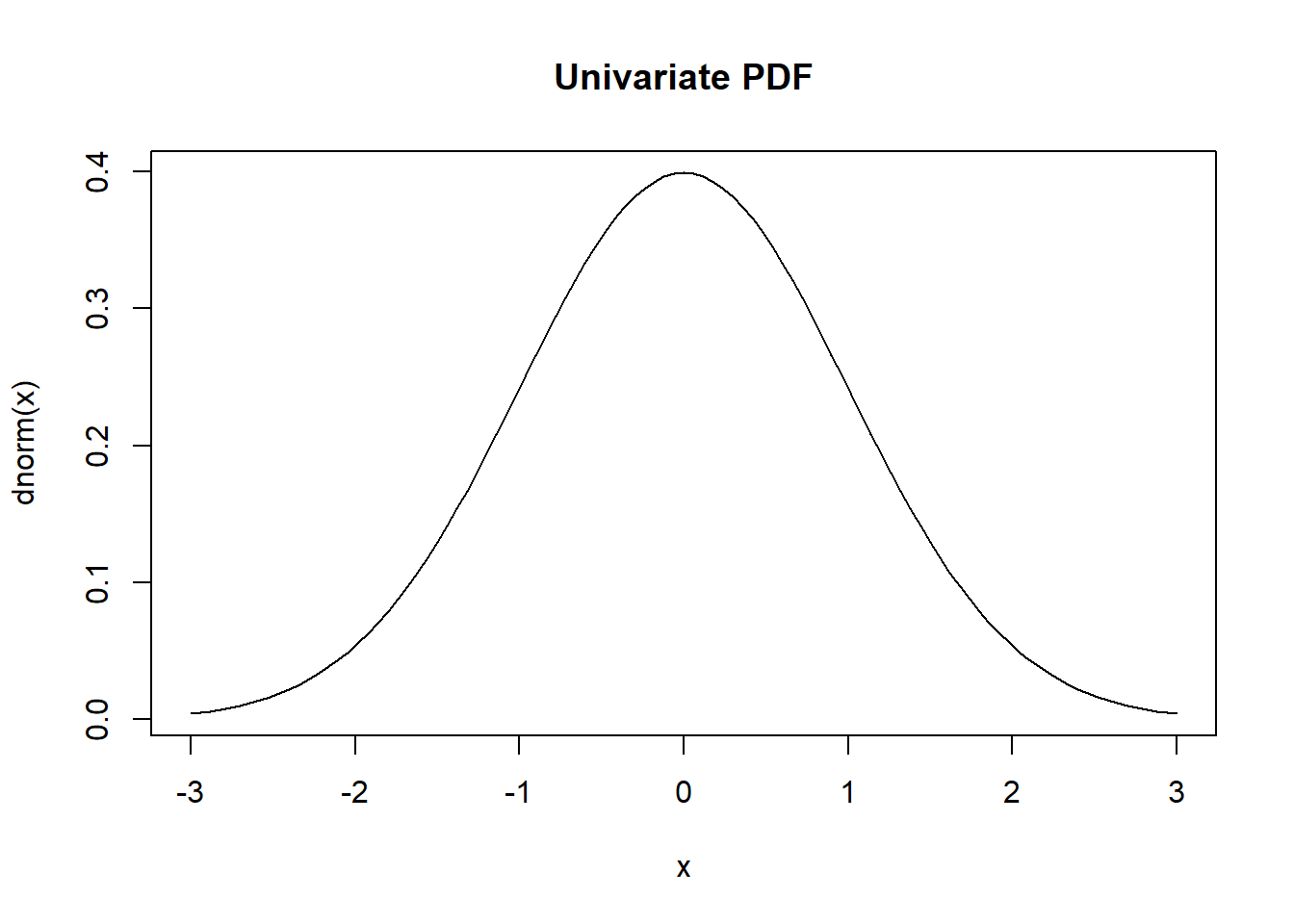
Code
def f(x):
  out = gamma.pdf(x,a=7,scale=12)*0.7 + gamma.pdf(x,a=7,scale=10)*0.2 + gamma.pdf(x,a=7,scale=11)*0.1
  return(out)

y = f(x)

import matplotlib.pyplot as plt

plt.plot(x, y)
plt.show()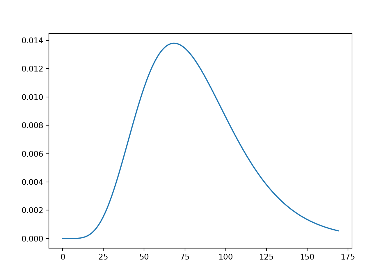
This resulting marginal distribution of 1st year salary is a mixture distribution. It represents the distribution of salaries ignoring information about industry.
Mixture distributions are highly useful. Many real-world phenomena can be described as a mixture. The distribution offers alot of flexibility when modeling.
The mystery CDF from above is a mixture distribution.
9.4 Middle and Spread
It is often useful to describe a distribution by its middle and spread. There are many ways to define the middle and spread.
| Middle | Spread |
|---|---|
| median | IQR |
| mean | variance |
| standard deviation | |
| Gini mean difference |
9.4.1 Median
In continous settings, the median is the value \(x*\) such that
\[ F(x*) = 0.5 \]
In the figure
It is the middle value in the sense that it splits the probability into equal halfs. There are some situations that require a slightly more complicated definition, like when CDF is not continuous or flat near the median.
9.4.2 Mean or Expected Value
The mean is another definition of middle, best understood in the context of the density.
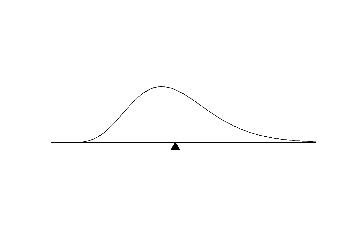
The mean is the point at which the density function would balance perfectly if it where placed on a fulcrum. It is the middle in the teeter-toter sense.
The mean can be calculated from the density using this formula:
\[ \text{mean} = E[X] = \int_{-\infty}^{\infty} x f_X(x) dx \]
The mean is also called the expected value of X or the expectation of X. Because the expected value of \(X\) is such an important quantity, it is often referred to by the single Greek letter \(\mu\).
\[ \mu = E[X] \]
More generally, the expectation of g(X) is the mean of the new random variable created by transforming X with function \(g\).
\[ \text{Expected value of } g(X) = E[g(X)] = \int_{-\infty}^{\infty} g(x) f_X(x) dx \]
Note that if \(g\) is not a linear operator, then
\[ E[g(X)] \neq g(E[X]) \]
For example, let \(g(x) = x^2\). Suppose \(X\sim N(0,1)\). Because \(g\) is not a linear operator,
\[ E[X^2] \neq \left(E[X]\right)^2 \]
As seen below, \(E[X] = 0\), and \((E[X])^2=0\), but 0 can’t be the mean of \(X^2\) because 0 is the minimum value of \(X^2\).
Code
import scipy.stats
X = scipy.stats.norm.rvs(size=1000000)
fig, (ax1, ax2) = plt.subplots(1, 2)
ax1.hist(X, bins=100, density=True)
ax2.hist(X**2, bins=100, density=True)

ax1.set_title("X ~ N(0,1)")
ax2.set_title("Z = X^2")
plt.tight_layout()
plt.show()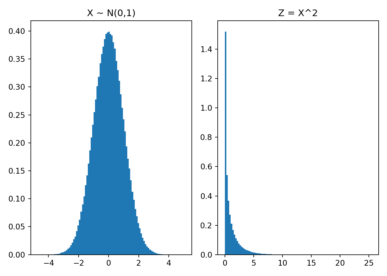
If \(g\) is a linear operator, like
\[ g(x) = a + b\cdot x, \]
then it is true that
\[ E[g(X)] = E[a + b\cdot X] = a + b\cdot E[X] = g\left(E[X]\right). \]
9.4.2.1 The sample average converges to the mean
It is common to summarize a sample of data with the sample average. For example, from a dataset with a blood pressure measurement from N=100 patients, one might calculate the average blood pressure with the usual formula:
\[ \text{sample average} = \sum_{i=1}^N \frac{1}{N} \text{blood pressure}_i \]
It turns out that, in most settings, if we keep sampling patients and measuring blood pressures and updating the sample average, then the sample average will converge to the distribution mean.
\[ \lim_{N\to\infty} \sum_{i=1}^N \frac{1}{N} \text{blood pressure}_i = \text{distribution mean} \]
In the figure below, we show this in action. Sampling from the distrubtion above, we see how the sample average is updated with every new draw. The blue line represents the distribution mean. As the number of samples increases, the sample average gets closer and closer to the blue line.
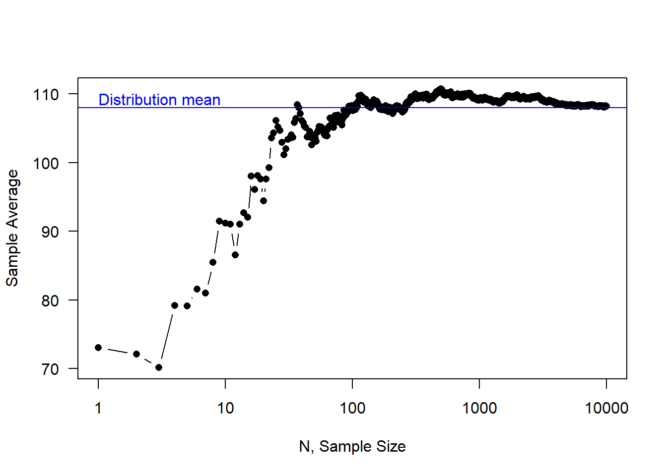
Note that this property is true even if we don’t know the underlying distribution. In the blood pressure example, the true population distribution may be complex or unknown. But the sample mean will almost surely converge to the mean of the underlying distribution.
Because this property is key to much of data science, it goes by a special name: the law of large numbers.
9.4.2.1.1 We can leverage the law of large numbers to calculate the mean of complex distributions
Even when we can write down the density function of the distribution, it may be difficult to calculate the mean. We can leverage the law of large numbers to calculate the mean. Much of Bayesian data analysis relies on this method.
The trick requires the ability to sample from the distribution.
Example. Suppose the variable \(Y\) has the following definition. It is possible that someone could calculate the mean of \(Y\) analytically, however, its mean is easily calculated using the law of large numbers.
\[ Y = \left(2 + \tan^{-1}(X)\right)^{1+ 0.2|X|}\quad \text{where } X \sim N(0,1) \]
We generate draws of X that follow the standard normal distribution, then we transform them according to the formula. To get a sense of the density, we generate the histogram.
Code
plt.close()
import scipy.stats
import numpy
N = 200000
X = scipy.stats.norm.rvs(size=N)
Y = (2 + numpy.arctan(X))**(1 + .2*numpy.abs(X))
plt.hist(Y, bins=100, density=True)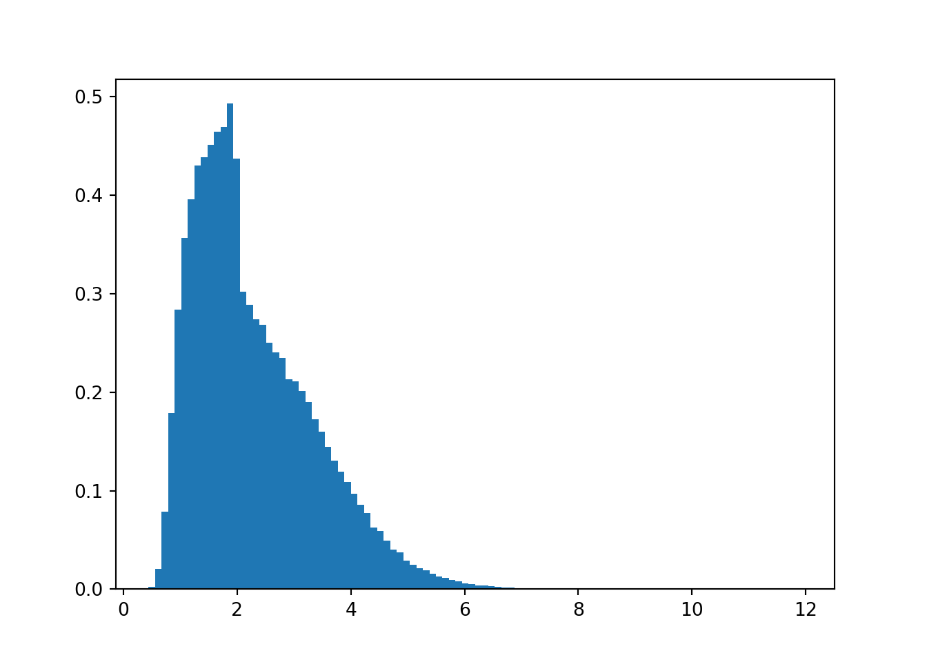
Ultimately, we calculate the sample average of a very large number of replicates to calculate, via simulation, the mean.
Code
Y.mean().item()2.2884829650327649.4.3 IQR
IQR stands for interquartile range and refers to the distance between the 0.75 quantile and the 0.25 quantile. It is a measure of spread. It is the width of the middle 50% of the mass.
Code
import scipy.stats
d = scipy.stats.norm
import matplotlib.pyplot as plt
import numpy
plt.close()
x = numpy.arange(-10,10,0.1)
fig, ((ax1, ax2), (ax3, ax4)) = plt.subplots(2, 2)
y1 = d.pdf(x)
y2 = d.pdf(x,scale=3)
y3 = d.cdf(x)
y4 = d.cdf(x,scale=3)
ax1.plot(x,y1)
ax1.plot([d.ppf(0.75), d.ppf(0.75)], [d.pdf(0), 0], color = "red")
ax1.plot([d.ppf(0.25), d.ppf(0.25)], [d.pdf(0), 0], color = "orange")
ax2.plot(x,y2)
ax2.plot([d.ppf(0.75, scale=3), d.ppf(0.75, scale=3)], [d.pdf(0, scale=3), 0], color = "red")
ax2.plot([d.ppf(0.25, scale=3), d.ppf(0.25, scale=3)], [d.pdf(0, scale=3), 0], color = "orange")
ax3.plot(x,y3)
ax3.plot([-10, d.ppf(0.75)], [0.75, 0.75], color = "red")
ax3.plot([d.ppf(0.75), d.ppf(0.75)], [0.75, 0], color = "red")
ax3.plot([-10, d.ppf(0.25)], [0.25, 0.25], color = "orange")
ax3.plot([d.ppf(0.25), d.ppf(0.25)], [0.25, 0], color = "orange")
ax4.plot(x,y4)
ax4.plot([-10, d.ppf(0.75, scale=3)], [0.75, 0.75], color = "red")
ax4.plot([d.ppf(0.75, scale=3), d.ppf(0.75,scale=3)], [0.75, 0], color = "red")
ax4.plot([-10, d.ppf(0.25, scale=3)], [0.25, 0.25], color = "orange")
ax4.plot([d.ppf(0.25, scale=3), d.ppf(0.25,scale=3)], [0.25, 0], color = "orange")
plt.tight_layout()
plt.show()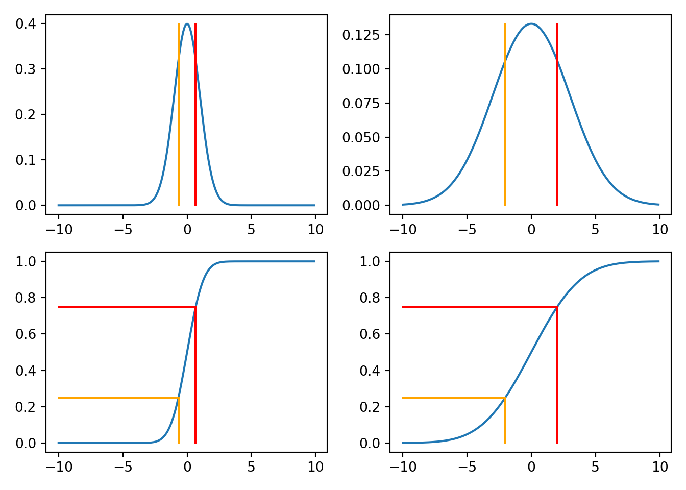
9.4.4 Variance
If \(\mu\) is the middle of the distribution, then
\[ x - \mu = \text{deviation from the mean.} \]
It might be tempting to calculate the expected deviation from the mean as a measure of spread, however, note that the deviations might be negative or positive. The positive and negative deviations will cancel out, and the expected deviation from the mean will be zero.
\[ E[\text{deviation from the mean}] = E[X-\mu] = E[X] - \mu = \mu - \mu = 0 \]
The fix, then, might be one of two options, \[ E[|X-\mu|] \text{ or } E[(X-\mu)^2], \]
the expected absolute deviation or the expected squared deviation. They are also called mean absolute deviation or mean squared deviation. Both are perfectly reasonable measures of spread. However, for mathematical ease, the expected squared deviation is more popular. (Its derivative is continuous which makes many of the mathematical derivations easier.)
The expected squared deviation is called the variance. It is a specific expectation.
\[ \text{variance of X} = V[X] = E[(X-\mu)^2] = E[X^2]-\left(E[X] \right)^2 \]
The expected absolute deviation is also used as a measure of spread, but it isn’t as popular.
9.4.5 Standard deviation
Consider the unit of measurement of the variance. If \(X\) is a measurement in meters, then the variance is in meters squared. It is often helpful to have a measurement of spread in the original outcome’s units.
The standard deviation is the square root of the variance. Its unit of measurement is the same as the original variable.
\[ \text{standard deviation} = \sqrt{V[X]} \]
9.4.6 Gini’s mean difference
Another approach to measuring spread is to consider two random draws from the distribution, say \(X_1\) and \(X_2\). Rather than focusing on deviation from the mean, one may consider the expected difference between two random draws \(X_1\) and \(X_2\),
\[ \text{mean absolute difference} = E[|X_1 - X_2|] \]
The mean absolute difference is called Gini’s mean difference.
9.4.7 Practice problems
- Website Conversion Rate: A marketing analyst models the conversion rate of a new landing page using a Beta(3, 7) distribution based on prior campaigns.
- What is the probability density that the true conversion rate is exactly 25%?
- What is the probability that the conversion rate exceeds 40%?
- Find the median conversion rate.
Code
# A
import scipy.stats
A = scipy.stats.beta.pdf(.25,3,7)
print(A)2.80316162109375Code
# B
B = 1 - scipy.stats.beta.cdf(.4,3,7)
print(B)0.23178700799999996Code
# C
C = scipy.stats.beta.ppf(.5,3,7)
print(C)0.2862366680227829- Baseball Batting Average: A baseball analyst models a rookie player’s true batting average using a Beta(81, 219) distribution (based on 300 at-bats with 81 hits).
- What is the probability that the player’s true batting average is between 0.250 and 0.300?
- Calculate the 90th percentile of the player’s batting average distribution.
- Project Completion: A project manager models the proportion of a software project completed by next Friday using a Beta(5, 2) distribution.
- What is the expected proportion completed?
- What is the probability that less than 60% will be completed?
- Adult Heights: Heights of adult men in a population follow a Normal(70, 3²) distribution (in inches).
- What proportion of men are taller than 6 feet (72 inches)?
- What height represents the 25th percentile?
- What is the probability a randomly selected man has a height between 68 and 74 inches?
Code
import scipy.stats

# A
A = 1-scipy.stats.norm.cdf(72, 70, 3)
print(A)0.2524925375469229Code
# B
B = scipy.stats.norm.ppf(.25, 70, 3)
print(B)67.97653074941175Code
# C
C = scipy.stats.norm.cdf(74,70,3) - scipy.stats.norm.cdf(68,70,3)
print(C)0.6562962427272092- Manufacturing Quality: A factory produces bolts with diameters following a Normal(10.0, 0.05²) mm distribution. Bolts must be between 9.9 and 10.1 mm to meet specifications.
- What percentage of bolts fail to meet specifications?
- If the factory produces 10,000 bolts per day, how many are expected to be rejected?
- What is the probability density at the target diameter of 10.0 mm?
- Standardized Test Scores: SAT Math scores follow approximately Normal(520, 115²) distribution.
- A scholarship requires a score in the top 10%. What is the minimum score needed?
- What is the probability a student scores between 500 and 650?
- If 5 students take the test independently, what is the probability all score above 600?
- Customer Service Times: The time (in minutes) to resolve a technical support call follows a Gamma(shape=3, rate=0.5) distribution.
- What is the probability a call takes longer than 10 minutes?
- What is the expected call duration?
- Find the 75th percentile of call duration.
Code
import scipy.stats

# A
A = 1-scipy.stats.gamma.cdf(10, a = 3, scale = 1/0.5)
print(A)0.12465201948308113Code
# B
# E[X] = shape * scale = shape / rate
B = 3 * (1/0.5)
print(B)6.0Code
# OR
scipy.stats.gamma.mean(a = 3, scale = 1/0.5)np.float64(6.0)Code
# OR (approximately)
scipy.stats.gamma.rvs(a = 3, scale = 1/0.5, size = 10000000).mean().item()5.999172788722289Code
# C
C = scipy.stats.norm.cdf(74,70,3) - scipy.stats.norm.cdf(68,70,3)
print(C)0.6562962427272092- Annual Rainfall: Annual rainfall (in inches) in a desert region follows a Gamma(shape=2, scale=3) distribution.
- What is the probability of receiving more than 9 inches of rain in a year?
- What is the probability of receiving between 3 and 6 inches?
- Calculate the median annual rainfall.
- Insurance Claims: The size of insurance claims (in thousands of dollars) follows a Gamma(shape=2.5, scale=4) distribution.
- What percentage of claims exceed $15,000?
- What is the probability density at a claim of $10,000?
- Find the claim amount such that 90% of claims are below this value.
- Server Downtime: The time between server failures follows an Exponential(rate=0.2) distribution (time in days).
- What is the probability the server runs for more than 7 days without failure?
- Given that the server has already run for 3 days, what is the probability it runs at least 5 more days?
- What is the median time between failures?
Code
import scipy.stats

# A
A = 1-scipy.stats.gamma.cdf(7, a = 1, scale = 1/0.2)
print(A)0.24659696394160646Code
# OR
A = 1-scipy.stats.expon.cdf(7,scale = 1/0.2)

# B
# Exponential is memoryless P(X > 8 | X > 3) = P(X > 5)
B = 1 - scipy.stats.expon.cdf(5, scale = 1/0.2)
print(B)0.36787944117144233Code
# OR
(1 - scipy.stats.expon.cdf(8, scale = 1/0.2))/(1 - scipy.stats.expon.cdf(3, scale = 1/0.2))np.float64(0.3678794411714423)Code
# C
C = scipy.stats.expon.ppf(.5, scale = 1/0.2)
print(C)3.4657359027997265- Customer Arrivals: Customers arrive at a coffee shop with time between arrivals following an Exponential(λ=4) distribution (time in minutes).
- What is the probability the next customer arrives within 30 seconds (0.5 minutes)?
- What is the probability that more than 2 minutes pass between consecutive customers?
- Find the 90th percentile of time between arrivals.
- Radioactive Decay: The time until the next decay event of a radioactive sample follows an Exponential(λ=0.05) distribution (time in seconds).
- What is the probability of waiting more than 30 seconds for the next decay?
- What is the expected waiting time?
- What is the probability density at t=20 seconds?
- Bus Arrival Window: During summer, a campus bus is equally likely to arrive at any time between 8:00 AM and 8:20 AM.
- A student shows up at 8:05 AM. What is the probability the bus arrives after they reach the stop?
- If the bus has not shown up by 8:05, what is the probability that the bus will show up by 8:15?
Code
import scipy.stats

# A
A = 1-scipy.stats.uniform.cdf(5, loc = 0, scale = 20)
print(A)0.75Code
# OR
1-scipy.stats.beta.cdf(5/20,a=1,b=1)np.float64(0.75)Code
# B
B = scipy.stats.uniform.cdf(15, loc = 5,  scale = 20 - 5)
print(B)0.6666666666666666Code
# OR P(T < 15 | T > 5) =  P(5 < T < 15) / P(T > 5)
(scipy.stats.uniform.cdf(15, loc = 0, scale = 20) - scipy.stats.uniform.cdf(5, loc = 0, scale = 20))/(1-scipy.stats.uniform.cdf(5, loc = 0, scale = 20))np.float64(0.6666666666666666)- Manufacturing Tolerance: A machine cuts wooden boards to a length that is equally likely to fall anywhere between 98.5 cm and 101.5 cm.
- What is the probability that a randomly selected board has length between 99.4 cm and 100.2 cm?
- What is the 90th percentile of board lenghts?
- Emergency Room Wait Times: At a small clinic, the wait time for non-urgent patients is modeled as Uniform(10, 40) minutes.
- What is the wait time threshold such that 90% of patients wait less than that time?
- Randomized Appointment Scheduling: A dentist randomly assigns check-up appointment start times uniformly over a 4-hour window from 8:00 AM to 12:00 PM.
- Create a plot of the PDF of appointment start time.
- Shade the portion of the PDF that corresponds to the probability of an appointment starting before 10:30 AM?
- What is the probability of an appointment between 9:30 and 10:45?
9.5 Joint Distribution of continuous random variables
Much of data science centers around predictions for an outcome \(Y\) based on observed values of predictors \(X_1\), …, \(X_d\). In the discrete chapter, we made predictions about preferred study location based on student status (graduate or undergraduate). Other predictors about location preference might include time of day (morning, afternoon, evening, late) or gender or major. You’ll recall from the discrete outcome chapter, organizing the joint probabilities into a table.
| Coffee Shop | Library | Dorm | |
|---|---|---|---|
| Undergraduate | 0.2 | 0.15 | 0.25 |
| Graudate | 0.2 | 0.15 | 0.05 |
The same information can be expressed as a surface.
In the continuous setting, we can do the same thing, discretizing the continuous variables. For example, if we have height and weight, we can discretize each into four bins. The bin heights represent the joint probabilities of the 16 possible outcomes.
Note that 4 bins was arbitrary; one could have used 10 bins.
Or 20 bins.
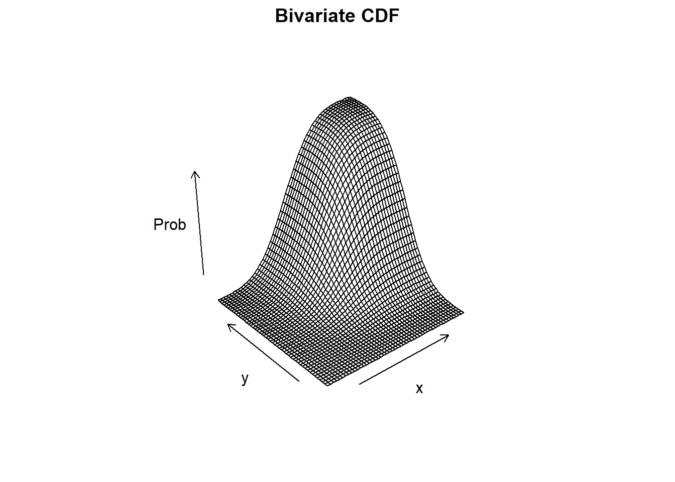
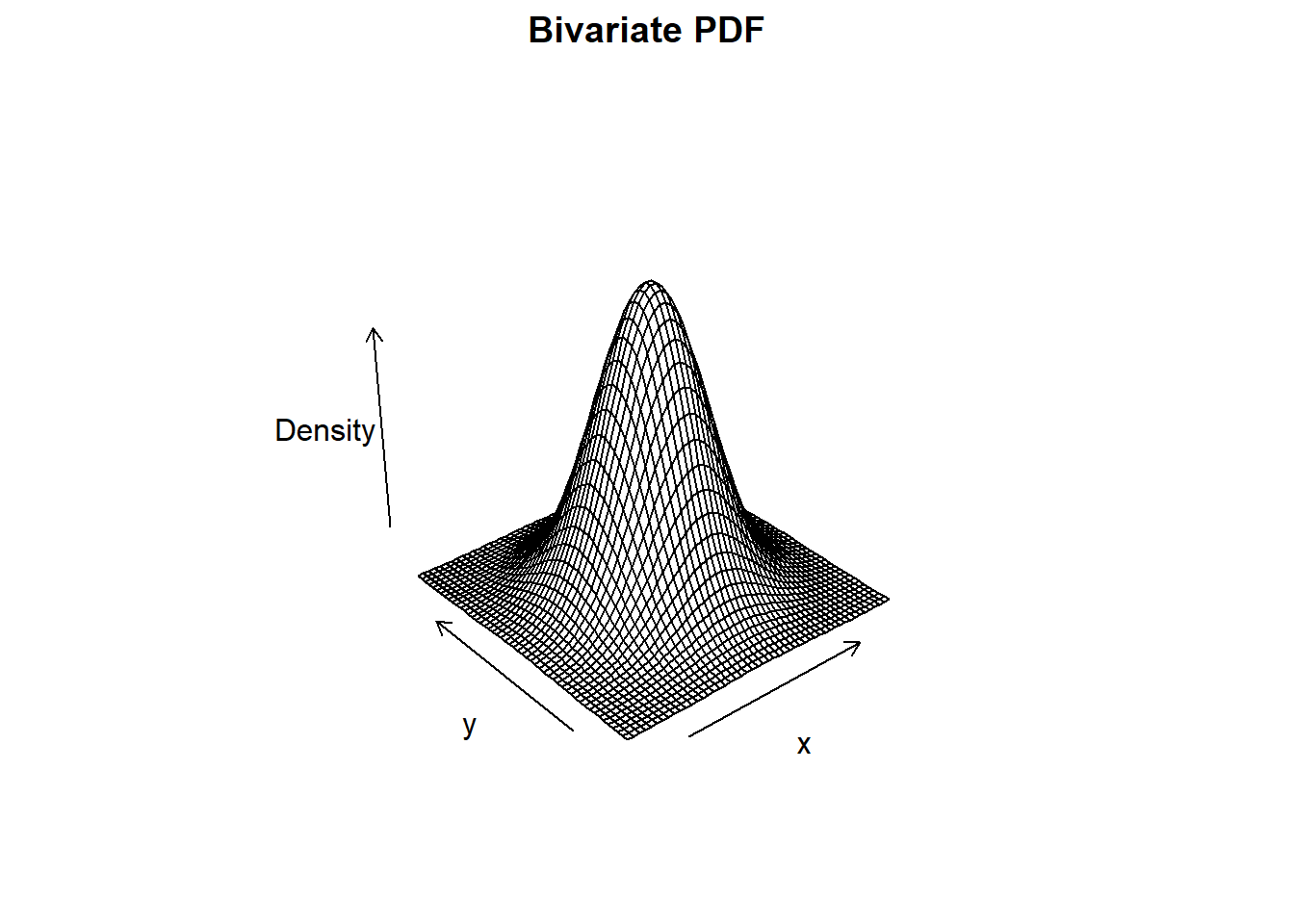
In the limit, the joint probabilities become joint densities.
The joint density becomes a surface which may be represented by a formula which takes values of of the two random variables and spits out the corresponding density.
\[ f:X\times Y \to Z \]
9.5.1 Example: Bivariate Normal
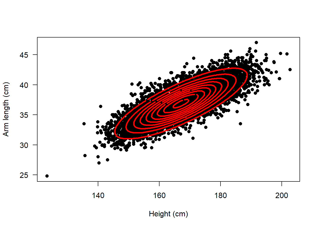
The normal distribution is commonly used in data science applications. Many applications involve examples of random outcomes which are well described by the bivariate normal distribution. For example, take height and arm measurements from an NHANES cycle.
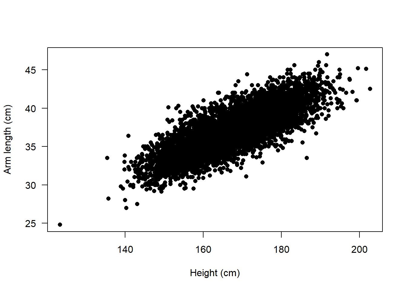
The points form a cloud that has a very oblong, symmetric structure.
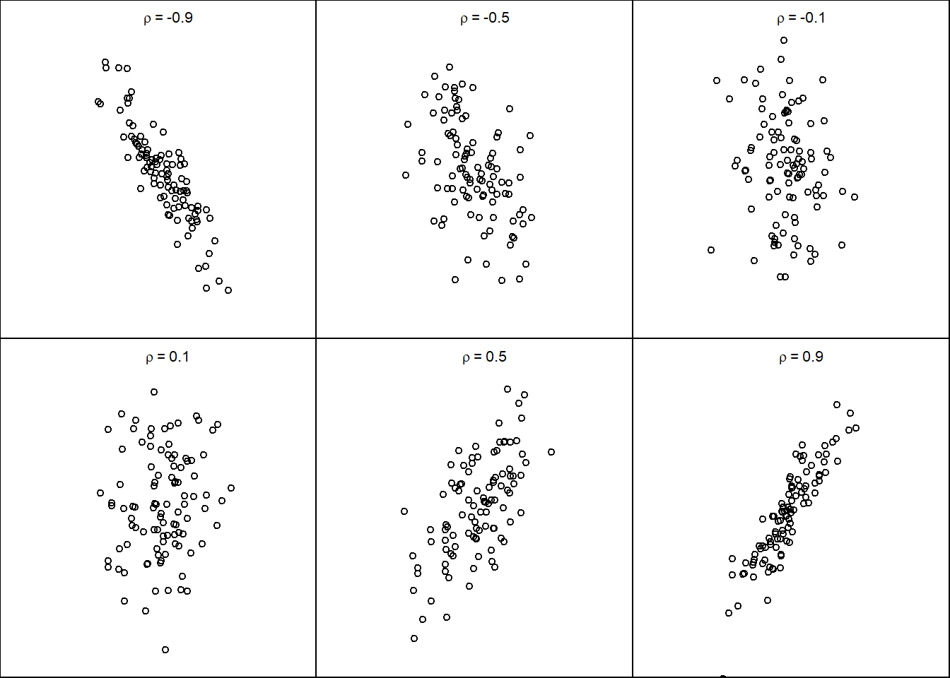
Depending on the relationship between the two random outcomes, the points might group tightly or might be spread out in a circular cloud. The figure below shows some different configuration of draws from the bivariate normal.
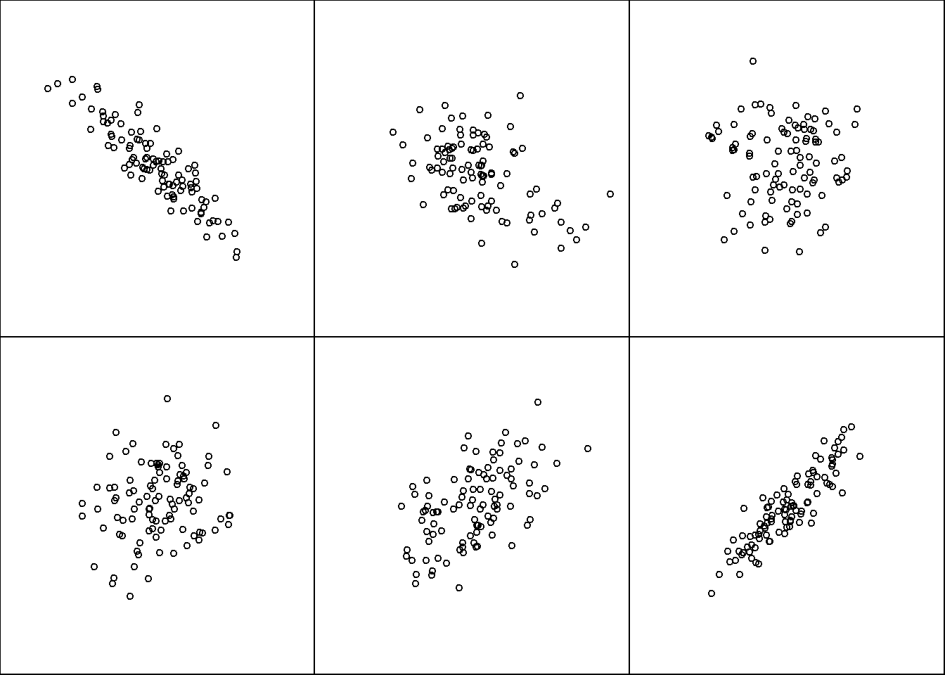
- What does the oblong, tight spread of points indicate?
- What would a spread out, circular cloud of points indicate?
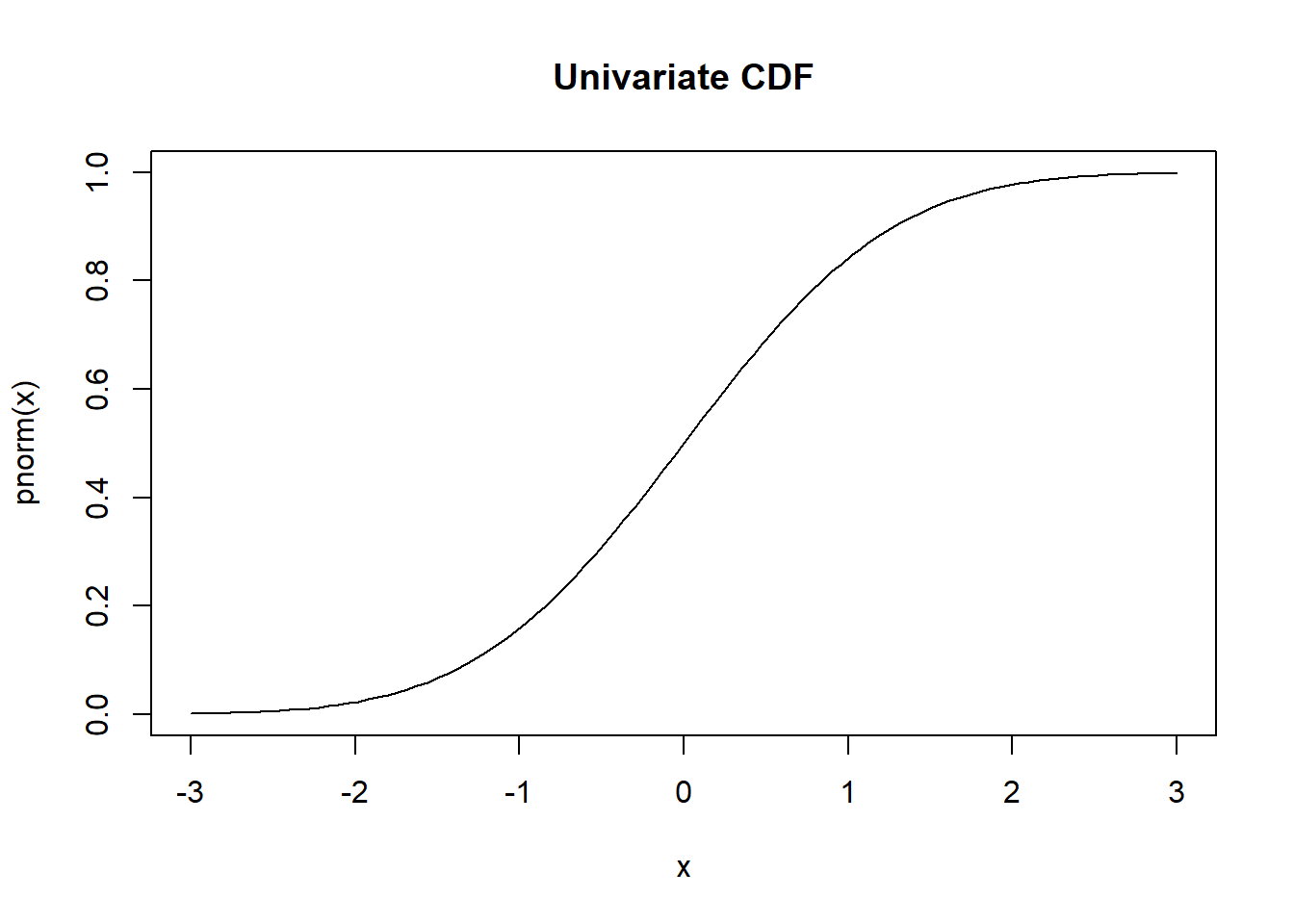
9.5.2 Univariate vs Bivariate
| Univariate | Bivariate | |
|---|---|---|
| CDF | \(F_X(x) = P(X\leq x)\) | \(F_{X,Y}(x,y) = P(X\leq x\ \text{and}\ Y\leq y)\) |
| \(f_X(x) = \frac{d}{dx} F_X(x)\) | \(f_{X,Y}(x,y) = \frac{\partial^2}{\partial x \partial y} F_{X,Y}(x,y)\) |

Interactive plot of PDF: (link)
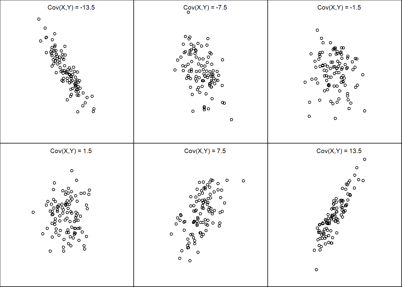
9.5.3 Covariance
A measure of linear association
\[ Cov(X,Y) = E[(X - E[X])(Y - E[y])]\]
\[ Cov(X,Y) = E[XY] - E[X]E[Y]\]
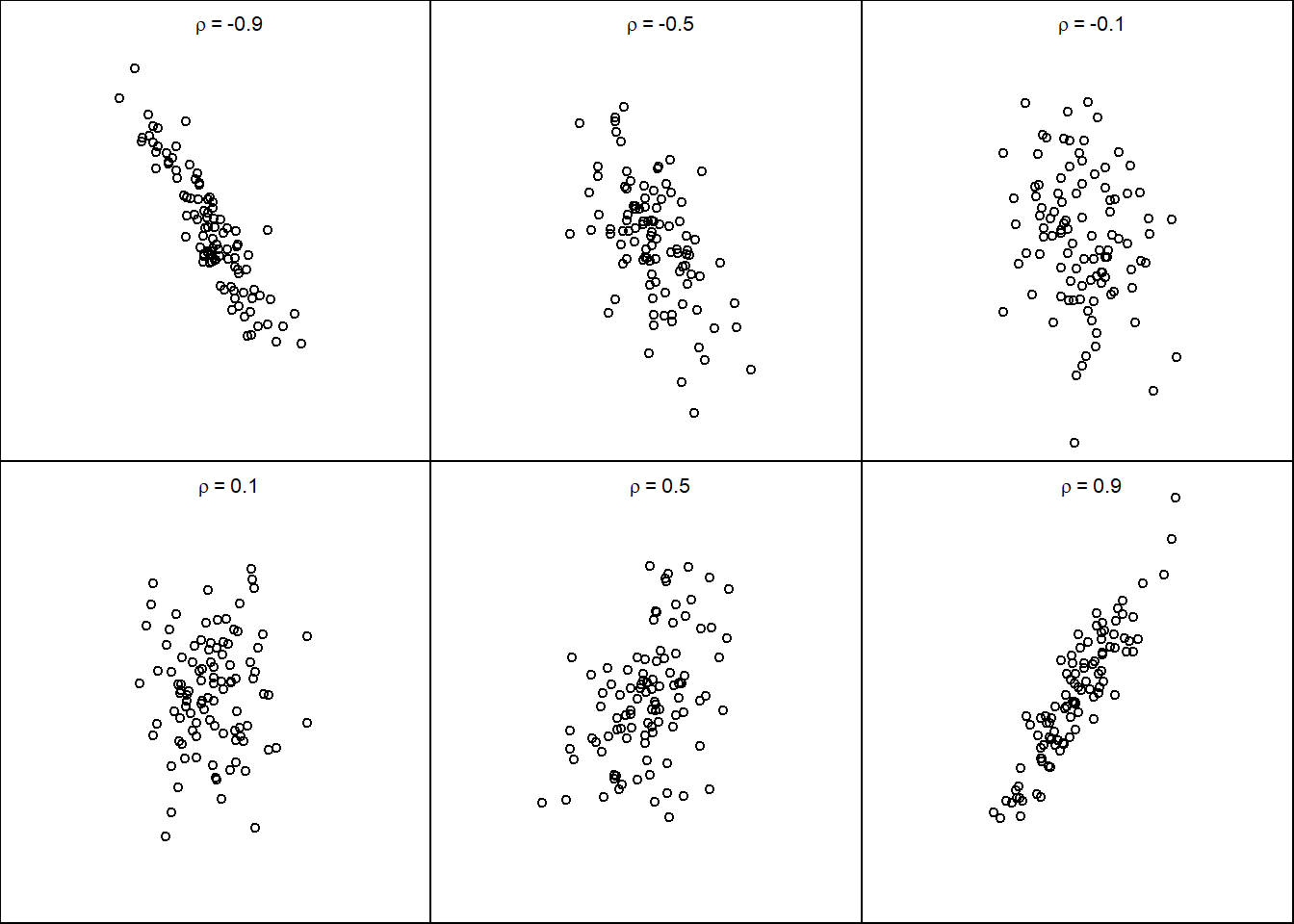
9.5.4 Correlation
A standardized measure of linear association
\[\rho(X,Y) = Cor(X,Y) = \frac{Cov(X,Y)}{\sqrt{V[X]V[Y]}}\]
A standardized measure of linear association
- \(-1\leq \rho(X,Y)\leq 1\)
- \(|\rho(X,Y)| = 1\) if and only if \(X\) and \(Y\) are exact linear functions of each other.
9.5.5 Example
Warning: Zero correlation is not independence