
Part 3: Estimation
In the part three, we tackle the problem of constructing models (or updating beliefs) from data. Because data collection is also a source of uncertainty, we investigate how to appropariately propagate the uncertainty to the inferences (aka, answers to our questions) that we pulled from the models. Communicating the uncertainty associated with our answers will be key.
The goal of estimation is to find a probability model that describes the collected data so that, ultimately, we can answer questions about a larger population.
There are several ways to use the data to estimate a probability model.
- Eyeball
- Kernel density estimation (nonparametric)
- Method of moments (parametric)
- Maximum likelihood (parametric)
- Bayesian posterior (parametric)
Eyeball isn’t really a formal method for estimating a probability model. But, it is a good place to start. The rest of part 3 will cover the formal methods in detail.
Fitting by Eye (Eyeball method)
The eyeball method involves looking at displays of the data and selecting or drawing a distribution function or density function which “looks good”. We demonstrate with examples.
Example: Pen Drop Data
Let’s consider data collected in class, in which students were asked to drop darts on a paper target. The distance from the strike to the center of the target was measured. Here we have 452 measurements.
Eyeball with Rayleigh distribution
Below is the ECDF of the pen drop data. Overlayed on the ECDF is the Rayleigh distribution function, which has a single parameter. Change the value of the parameter through the slider so that the Rayleigh distribution function matches, as best it can, the data.
Eyeball with gamma distribution
Below is the same data, overlayed with the gamma distribution function, which has two parameters. Change the value of the parameters through the slider so that the gamma distribution function matches, as best it can, the data.
Eyeball with Weibull distribution
Below is the same data, overlayed with the Weibull distribution function, which has two parameters. Change the value of the parameters through the slider so that the distribution function matches, as best it can, the data.
Example: Infant birthweight data
Eyeball with kernel density estimation
Below is infant birthweight data. Overlayed is a special type of mixture distribution, known as a kernel density. This distribution function is controlled by a smoothing parameter and the type of kernel. Change the kernel by clicking different kernel types. Change the value of the smoothing parameter through the slider. Pick ther kernel and smoothing parameter combination so that the distribution function is a good description of the data.
In class exercise
- Create a group report by taking a snapshot of the figures above with your best model fit by eye.
- Reflect on your process for fitting by eye:
- What features did you consider as you selected parameters by eye?
- Propose a way to quantify a better or worse fit.
Parametric vs Nonparametric
A parametric distribution is one whose shape or mathematical expression is determined by a finite, fixed number of parameters. Take the normal distribution as an example. Its shape is determined by parameters \(\mu\) and \(\sigma\). One can change these values to change the location and spread.
The mathematical expression for the pdf includes \(\mu\) and \(\sigma\):
\[ f(x, \mu, \sigma) = \frac{1}{\sqrt{2\pi\sigma^2}}e^{-\frac{(x-\mu)^2}{2\sigma^2}} \]
Even a mixture distribution has a finite, fixed number of parameters. The mixture of three normals shown below has 8 parameters: 3 \(\mu\)s, 3 \(\sigma\)s, and 2 \(\pi\)s. The additional parameters result in a distribution that can take on a wider variety of shapes compared to a single, normal random variable.
In contrast, a nonparametric distribution is constructed from data, and the number of parameters is determined by the size of the data. The number of parameters is not fixed.
The empirical cumulative density function (ECDF) is an example of a nonparametric distribution function. It is constructed from data, and the number of parameters is \(u-1\) where \(u\) is the number of unique values in the dataset.
Code
Hmisc::getHdata(nhgh)
`%||%` <- function(a,b) paste0(a,b)
If we look at first 100 BMIs in the NHANES data, we see 97 unique jumps.
plot(ecdf(nhgh$bmi[1:100]), main = "ECDF of BMI, N=" %||% 100, xlab = "BMI", xlim = c(0,80))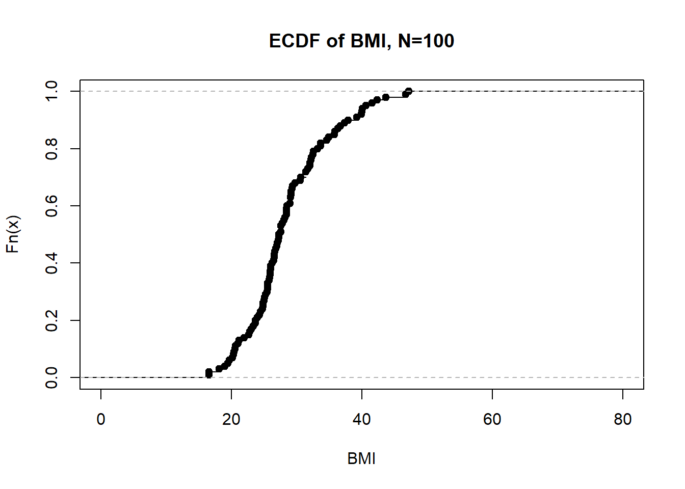
If we look at all the BMIs in the NHANES data, there are 2389 unique jumps for 2388 parameters.
n <- sum(!is.na(nhgh$bmi))
plot(ecdf(nhgh$bmi), main = "ECDF of BMI, N=" %||% n, xlab = "BMI", xlim = c(0,80))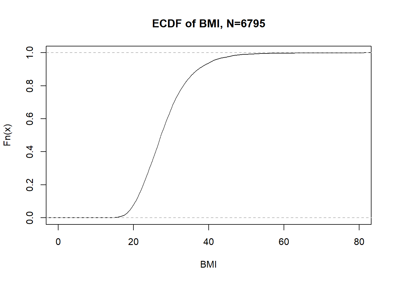
Note: Non-parametric doesn’t mean no parameters; it simply means the number of parameters is determined from the data and potentially very large.