import numpy as np
np.random.seed(1)
3*np.sqrt(-2*np.log(1-np.random.uniform(size=10)))
array([3.1165534 , 4.78897218, 0.04537471, 2.54562951, 1.69019902,
1.32057173, 1.92615249, 2.76253085, 3.01631327, 3.73246245])This assignment will be due Friday, Dec 12 at 11:59 PM. This assignment will be graded for accuracy.
We will review the exam in class on Tuesday, Dec 9 and during office hours.
Some solutions will be posted Friday, Dec 12 at 9:00 AM.
This practice exam primarily covers the material covered in the course since exam 2. The final exam is cumulative, and you are encouraged to also review the previous exams and exam preps.
Some questions will require you to compute, simulate, or plot things—tasks that cannot be completed during the exam. However, since this is also a homework assignment, you should complete those tasks as part of your practice. While the exam will not require you to use a computer, you may be asked to read and understand code, just as you were on exams 1 and 2.
Q1 What is a random variable? Explain the difference between a random variable and a regular variable you might use in algebra.
Q2 What distinguishes a continuous random variable from a discrete random variable?** Give an example of each.
Q3 What is a cumulative distribution function (CDF)? What are its inputs and what values does it return?
Q4 How would you use the probability density function (PDF) to find P(a < X < b)?
Q5 Explain the relationship between a PDF and a CDF. How would you calculate one from the other?
Q6 The probability density function for an exponential distribution with rate parameter λ is:
\[ f(x) = \lambda e^{-\lambda x}, \quad x \geq 0 \]
Suppose buses arrive at a bus stop according to an exponential distribution with rate λ = 0.5 per minute. This means the average waiting time is 1/λ = 2 minutes.
(A) Write Python code using scipy.stats.expon to plot the PDF of the exponential distribution with rate λ = 0.5. On the same plot, add the PDF for an exponential distribution with rate λ = 1.0 (scale = 1).
(B) What is the average waiting time for both distributions?
The normal distribution is characterized by two parameters: mean μ (mu) and standard deviation σ (sigma).
Q7 The probability density function for a normal distribution is:
\[ f(x) = \frac{1}{\sigma\sqrt{2\pi}} e^{-\frac{1}{2}\left(\frac{x-\mu}{\sigma}\right)^2} \]
(A) Let the mean μ = 50 and standard deviation σ = 10. Plot the density.
(B) Generate N=100 values from a Normal(50, 10) distribution. What proportion of your sample falls within one standard deviation of the mean (between 40 and 60)?
(C) The theoretical proportion is 68%. Calculate the simulation error (absolute difference).
(D) Repeat (B) and (C) 10,000 times. Create a histogram of the simulation error with 100 bins.
(E) Repeat (D) with N=1000. Create a plot which overlays the histogram of the simulartion errors from part (D) and part (E).
(F) What do the differences in the histograms in part (E) indicate?
Q8 The probability density function for a gamma distribution with shape parameter k and rate parameter λ is:
\[ f(x) = \frac{\lambda^k}{\Gamma(k)} x^{k-1} e^{-\lambda x}, \quad x \geq 0 \]
The gamma distribution is often used to model waiting times for multiple events. If individual events occur according to an exponential distribution with rate λ, then the time until the k-th event follows a gamma distribution.
(A) In a single figure, plot the density functions when λ=1 and k=1, 2, 3, and 5.
(B) Describe how the shape of the distribution changes as k increases.
(C) Generate 10,000 random samples from a Gamma(5, 2) distribution. Calculate the sample mean. How does it compare to the theoretical mean k/λ = 5/2 = 2.5?
(D) Create a histogram with 100 bins of your simulated values and overlay the theoretical PDF. Do they match?
Q9 The probability density function for a beta distribution with shape parameters α (alpha) and β (beta) is:
\[ f(x) = \frac{\Gamma(\alpha + \beta)}{\Gamma(\alpha)\Gamma(\beta)} x^{\alpha-1} (1-x)^{\beta-1}, \quad 0 \leq x \leq 1 \]
The beta distribution is defined on the interval [0, 1], making it useful for modeling proportions, probabilities, and percentages.
(A) On the same plot, show beta distributions with α = β = 1, α = β = 2, and α = β = 5.
(B) In the same figure, plot Beta(2, 5) and Beta(5, 2).
(C) Comparing the plots in (A) and (B), what happens when α = β? Describe the shape. What happens when α > β? Describe the shape.
Q10 A mixture distribution combines two or more probability distributions. The PDF of a mixture is:
\[ f(x) = w_1 f_1(x) + w_2 f_2(x) + \cdots + w_k f_k(x) \]
where \(w_i\) are weights (mixing proportions) that sum to 1, and \(f_i(x)\) are the component densities.
(A) Give an example of a real-world situation where a mixture distribution might be appropriate.
(B) Generate 10,000 samples from the mixture of two normals: 23: 0.6×Normal(20, 3) + 0.4×Normal(30, 2). (Hint: Approach: For each sample, first randomly decide which component (1 or 2) based on the weights, then draw from that component.) Create a histogram and overlay the theoretical mixture density.
Q11 Expected Value and Variance.
(A) What does the expected value (mean) of a random variable represent?
(B) For a continuous random variable X with density f(x), write the formula for E[X].
(C) For a continuous random variable X with density f(x), write the formula for and E[X²]?
(D) Write the formula for Var(X) in terms of E[X] and E[X²].
(E) What is the relationship between variance and standard deviation?
(F) What is an advantage of the standard deviation compared to the variance?
Q12 Suppose X has density function f(x) = 2x for 0 ≤ x ≤ 1, and f(x) = 0 otherwise.
(A)Calculate E[X] using the integral formula.
(B) Calculate E[X²].
(C) Calculate Var(X).
Q13 If you have a function g(x) that has the right shape for a density (g(x)>0) but doesn’t integrate to 1, how do you find the normalizing constant c so that c·g(x) is a valid PDF?
Q14 Suppose we have f(x) = c·x² for 0 ≤ x ≤ 2, and f(x) = 0 otherwise. Find the value of c that makes this a valid probability density function.
Q15 Consider f(x) = c·e^(-x) for x ≥ 1. Find the normalizing constant c.
Q16 Suppose X has density f(x) = 3x² for 0 ≤ x ≤ 1. Calculate P(0.25 < X < 0.75) by integration.
Q17 The following data are believed to be from the Rayleigh distribtuion,
\[ f(x) = \frac{x}{\theta} e^{-\frac{x^2}{2\theta}}\qquad x\geq 0 \]
import numpy as np
np.random.seed(1)
3*np.sqrt(-2*np.log(1-np.random.uniform(size=10)))array([3.1165534 , 4.78897218, 0.04537471, 2.54562951, 1.69019902,
1.32057173, 1.92615249, 2.76253085, 3.01631327, 3.73246245])(A) Calculate the maximum likelihood estimate of \(\theta\).
(B) Create a plot of the estimated density function.
(C) With the estimated distribution, calculate \(P(X\leq 1)\).
Q18 Consider a system composed of two sensors, A and B, in sequence.

The system fails when either A or B fails. The failure time for sensor A follows an exponetial distribution with mean failure time of 3 years. The failure time for sensor B follows a Weibull distrubtion with scale = 3 and shape = 2.
import scipy.stats as st
import matplotlib.pyplot as plt
import numpy as np
xx = np.arange(0,10,0.1)
zz = st.expon.pdf(xx,scale=3)
yy = st.weibull_min.pdf(xx, c = 2, scale = 3)
plt.close()
plt.plot(xx,zz, label = "Sensor A")
plt.plot(xx,yy, label = "Sensor B")
plt.xlabel("Failure time (years)")
plt.ylabel("Density")
plt.legend()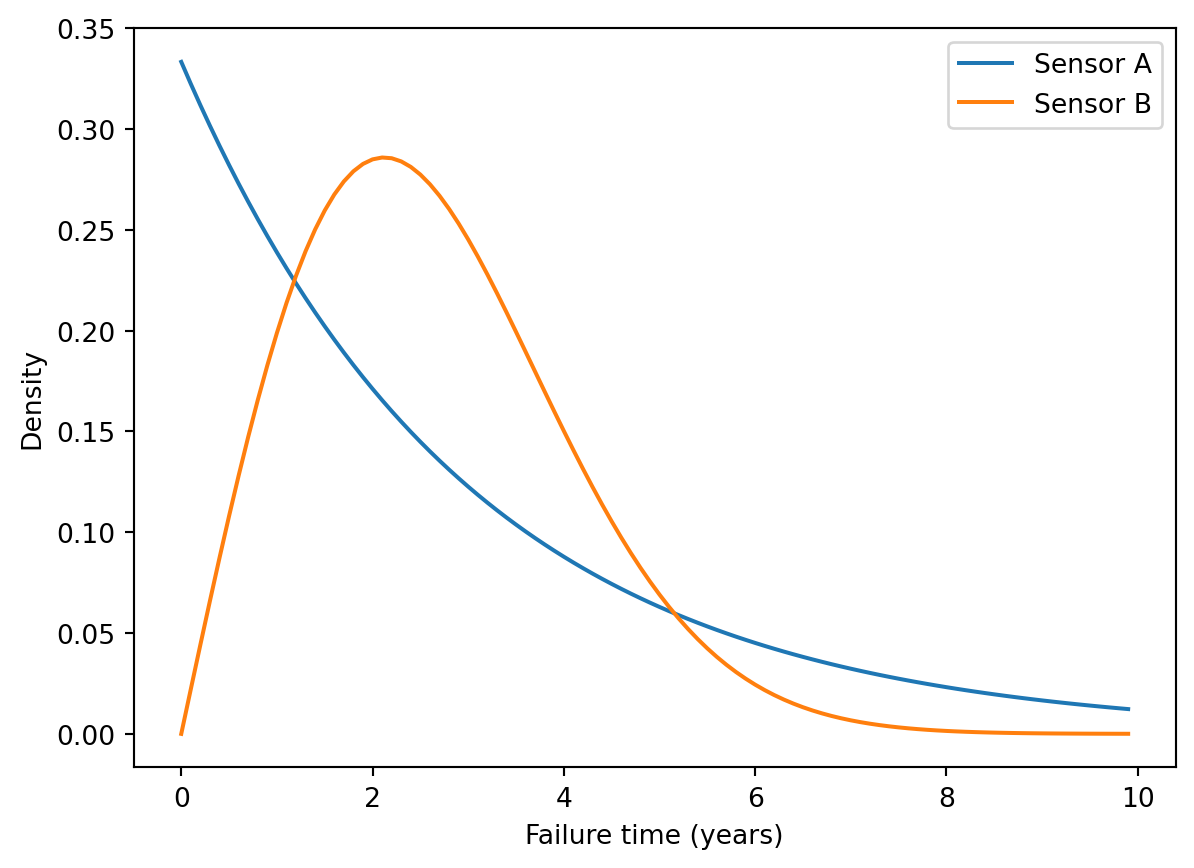
If \(A_F\) and \(B_F\) are the failure times of sensors \(A\) and \(B\), then the failure time of the entire system, denoted by \(S_F\) is
\[ S_F = \min\left(A_F, B_F\right) \]
We can simulate the distrubtion of \(S_F\) and its properties like mean, median, and variance.
R = 10000
AF = st.expon.rvs(size=R,scale=3)
BF = st.weibull_min.rvs(size=R, c = 2, scale = 3)
SF = np.minimum(AF, BF)
plt.close()
plt.hist(SF, density = True,bins=100)
plt.close()
Summary = {
      "Mean":f"{SF.mean().item():.2f} (years)"
    , "Median":f"{np.median(SF).item():.2f} (years)"
    , "SD":f"{np.std(SF).item():.2f} (years)"
    , "Var":f"{np.var(SF).item():.2f} (years^2)"
}
Consider an improvement of the system, in which additional sensors are added in parallel.

The new system fails either when all of the A sensors fail or when all of the B sensors fail. The failure time of the sensors are all independent.
(A) Using simulation, generate a density estimate of the failure time for the improved system using the histogram. (Compare it to the previous distribution by placing the histograms of the old and new systems in the same plot.)
(B) Add another column to the table of summary measures for the improved system.
(C) Create a single figure with the eCDF of both systems. Be sure to include a legend or labels.
Q19 Ball bearings from machine A have diameters which follow a normal distribution with mean 10 and standard deviation 0.1. Machine B is more precise and generates ball bearings with the same mean but with a smaller standard deviation of 0.025. The additional precision comes at a cost: for every 1 ball bearing generated by machine B, machine A is able to produce 2 bearings.
(A) Generate a plot of the marginal density of ball bearing diameters generated at the factory. (The factory only has machines A and B.)
(B) Calculate the probability that a randomly selected ball bearing came from machine B given that its diameter is 9.9.
Q20 The Monte Hall problem is a classic game show. Contestants on the show where shown three doors. Behind one randomly selected door was a sportscar; behind the other doors were goats.
At the start of the game, contestants would select a door, say door A. Then, the host would open either door B or C to reveal a goat. At that point in the game, the host would ask the contestant if she would like to change her door selection. Once a contestant decided to stay or change, the host would open the chosen door to reveal the game prize, either a goat or a car.
Consider two strategies:
(A) Use simulation to determine the probability that each strategy wins the sportscar. The following code will simulate a single game. You may want to tweak it so that it generates results for R replicates.
initial_choice = 1
car_door = np.random.randint(1, 3+1, size=1)
stay_win = 1*(car_door == initial_choice)
switch_win = []
for i in range(1):
    if car_door[i] == initial_choice:
        switch_win.append(0)
    else:
        switch_win.append(1*(np.random.randint(1, 3-1, size=1).item() == 1))
out = {"Stay":stay_win, "Switch":switch_win}
print(out)
{'Stay': array([0]), 'Switch': [1]}(B) Modify the code so that it works for a game with \(N\) doors. Calculate the probability of winning for each strategy with \(N=4\).