Final Exam Prep Selected Solutions

Q6 The probability density function for an exponential distribution with rate parameter λ is:

\[ f(x) = \lambda e^{-\lambda x}, \quad x \geq 0 \]

Suppose buses arrive at a bus stop according to an exponential distribution with rate λ = 0.5 per minute. This means the average waiting time is 1/λ = 2 minutes.

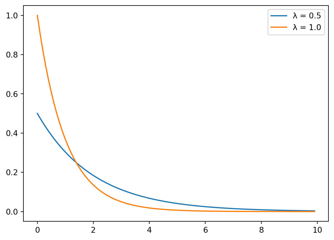
(A) Write Python code using scipy.stats.expon to plot the PDF of the exponential distribution with rate λ = 0.5. On the same plot, add the PDF for an exponential distribution with rate λ = 1.0 (scale = 1).

import scipy.stats as st
import matplotlib.pyplot as plt
import numpy as np

x = np.arange(0,10,0.1)
y = st.expon.pdf(x, scale = 1/0.5)
plt.close()
plt.plot(x,y, label = "λ = 0.5")

y2 = st.expon.pdf(x, scale = 1/1)
plt.plot(x,y2, label = "λ = 1.0")
plt.legend()

Q7 The probability density function for a normal distribution is:

\[ f(x) = \frac{1}{\sigma\sqrt{2\pi}} e^{-\frac{1}{2}\left(\frac{x-\mu}{\sigma}\right)^2} \]

(B) Generate N=100 values from a Normal(50, 10) distribution. What proportion of your sample falls within one standard deviation of the mean (between 40 and 60)?

y = st.norm.rvs(loc=50,scale=10,size=100,random_state = 1)
observed_proportion = ((40 < y) & (y <= 60)).mean()
print(observed_proportion)
0.76

(C) The theoretical proportion is 68%. Calculate the simulation error (absolute difference).

true_proportion = st.norm.cdf(60,50,10) - st.norm.cdf(40,50,10)
sim_error = np.abs(observed_proportion - true_proportion)
print(sim_error)
0.07731050786291416

(D) Repeat (B) and (C) 10,000 times. Create a histogram of the simulation error with 100 bins.

def sim(n):
    y = st.norm.rvs(loc=50,scale=10,size=n)
    observed_proportion = ((40 < y) & (y <= 60)).mean()
    true_proportion = st.norm.cdf(60,50,10) - st.norm.cdf(40,50,10)
    sim_error = np.abs(observed_proportion - true_proportion)
    return sim_error
out = [sim(100) for i in range(10000)]
plt.close()
junk = plt.hist(out, bins = 100, density=True)
plt.show()

(E) Repeat (D) with N=1000. Create a plot which overlays the histogram of the simulartion errors from part (D) and part (E).

out2 = [sim(1000) for i in range(10000)]
plt.close()
plt.hist(out, bins = 100, density=True, label = "N=100")
junk = plt.hist(out2, bins = 100, density=True, label = "N=1000")
plt.show()

(F) What do the differences in the histograms in part (E) indicate?

The simulation error, on average, is much smaller when N is 1000.

print("Avg sim error N=100:  ", f'{np.mean(out):.4f}')
print("Avg sim error N=1000: ", f'{np.mean(out2):.4f}')
Avg sim error N=100:   0.0378
Avg sim error N=1000:  0.0117

Q12 Suppose X has density function f(x) = 2x for 0 ≤ x ≤ 1, and f(x) = 0 otherwise.

(A)Calculate E[X] using the integral formula.

\[ \begin{align*} E[X] &= \int x f(x)\, dx \\ &= \int_0^1 x 2x\, dx \\ &= 2\int_0^1 x^2\, dx \\ &= 2\left. \frac{x^3}{3} \right|_0^1 \\ &=2\frac{(1)^3}{3} - 2\frac{(0)^3}{3} \\ &=\frac{2}{3}\\ \end{align*} \]

(B) Calculate E[X²].

\[ \begin{align*} E[X^2] &= \int x^2 f(x)\, dx \\ &= \int_0^1 x^2 2x\, dx \\ &= 2\int_0^1 x^3\, dx \\ &= 2\left. \frac{x^4}{4} \right|_0^1 \\ &=2\frac{(1)^4}{4} - 2\frac{(0)^4}{4} \\ &=\frac{2}{4}\\ &=\frac{1}{2}\\ \end{align*} \]

(C) Calculate Var(X).

\[ \begin{align*} V[X] &= E[X^2] - \left(E[X]\right)^2 \\ & = \frac{1}{2} - \left(\frac{2}{3}\right)^2 \\ & = \frac{1}{2} - \frac{4}{9} \\ & = \frac{9}{18} - \frac{8}{18} \\ & = \frac{1}{18}\\ \end{align*} \]

# BONUS: Calc variance with sim
# generate draws from dist
x = np.sqrt(np.random.uniform(size=10000))
plt.close()
plt.hist(x, density=True, bins=100)
sim_var = x.var()
print(" Analytic var: ",f'{1/18:.4f}' , "\n Sim var: ", f'{sim_var:.4f}', "\n Difference: ", f'{np.abs(sim_var-1/18):.4f}' )
 Analytic var:  0.0556 
 Sim var:  0.0564 
 Difference:  0.0009

Q17 The following data are believed to be from the Rayleigh distribtuion,

\[ f(x) = \frac{x}{\theta} e^{-\frac{x^2}{2\theta}}\qquad x\geq 0 \]

import numpy as np
np.random.seed(1)
d1 = 3*np.sqrt(-2*np.log(1-np.random.uniform(size=10)))

(A) Calculate the maximum likelihood estimate of \(\theta\).

Strategy:

  1. Construct likelihood function, \({\cal L}(\theta)\)
  2. Construct log likelihood function, \(\ell(\theta) = \log {\cal L}(\theta)\)
  3. Find maximum by calculating derivative and finding root
  4. (Not shown) Verify solution is maximum
  5. Plug-in data to calculate estimate based on observed values

Step 1 \[ \begin{align*} {\cal L}(\theta) &= \prod_{i=1}^n f(x_i\mid\theta)\\ &=\prod_{i=1}^n \frac{x_i}{\theta} e^{-\frac{x_i^2}{2\theta}}\\ \end{align*} \]

Step 2

Recall a few properties of \(\log(x)\).

  1. \(\log(ab) = \log(a) + \log(b)\)
  2. \(\log(a^b) = b\log(a)\)
  3. \(\log(e^a) = a\)

\[ \begin{align*} \ell(\theta) &= \log \left(\prod_{i=1}^n f(x_i\mid\theta)\right)\\ &=\sum_{i=1}^n \log\left(\frac{x_i}{\theta} e^{-\frac{x_i^2}{2\theta}}\right)\\ &=\sum_{i=1}^n \log\left(x_i\right) -\log(\theta) + \log\left(e^{-\frac{x_i^2}{2\theta}}\right)\\ &=\sum_{i=1}^n \log\left(x_i\right) -\log(\theta) -\frac{x_i^2}{2\theta}\\ \end{align*} \]

Step 3

\[ \begin{align*} \frac{d}{d\theta}\ell(\theta) &= \sum_{i=1}^n 0 - \frac{1}{\theta} -\frac{x_i^2}{2\theta^2}(-1)\\ &= \sum_{i=1}^n-\frac{1}{\theta}+ \frac{x_i^2}{2\theta^2}\\ &= -\frac{n}{\theta}+ \frac{1}{2\theta^2}\sum_{i=1}^n x_i^2\\ &= -\frac{n}{\theta}+ \frac{1}{2\theta^2}\frac{n}{1}\left(\frac{1}{n}\sum_{i=1}^n x_i^2\right)\\ &= -\frac{n}{\theta}+ \frac{n}{2\theta^2}\overline{x^2}\\ \end{align*} \]

\[ \begin{align*} -\frac{n}{\theta}+ \frac{n}{2\theta^2}\overline{x^2} &\overset{set}{=} 0\\ \frac{\theta^2}{n}\left(-\frac{n}{\theta}+ \frac{n}{2\theta^2}\overline{x^2}\right) &= \frac{\theta^2}{n} \cdot 0\\ \left(-\frac{n\theta^2}{n\theta}+ \frac{n\theta^2}{n2\theta^2}\overline{x^2}\right) &= 0\\ -\theta + \frac{1}{2}\overline{x^2} &= 0\\ \theta &= \frac{1}{2}\overline{x^2}\\ \end{align*} \]

Step 5

theta_hat = np.mean(d1**2)/2 
print("Estimate θ: ", f'{theta_hat:.3f}')
Estimate θ:  3.905

(B) Create a plot of the estimated density function.

def f(x,theta):
    return x/theta*np.exp(-x**2/2/theta)

xx = np.arange(0, 10, .1)
yy = f(xx,theta_hat)
plt.close()
plt.plot(xx,yy)

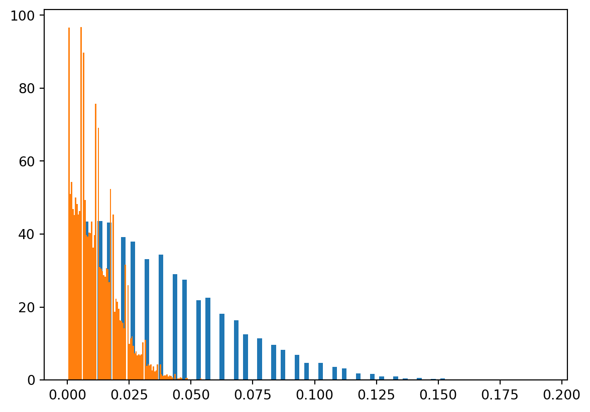
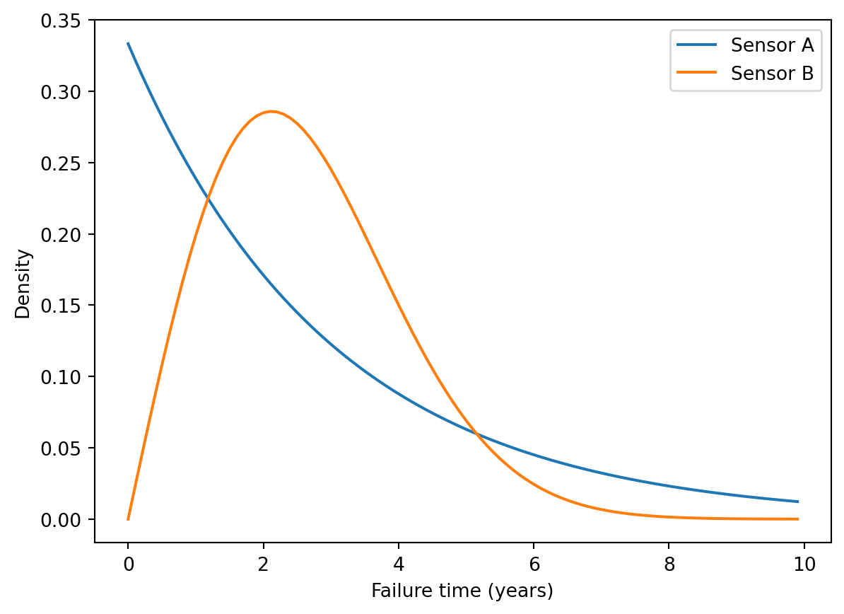
Q18 Consider a system composed of two sensors, A and B, in sequence.

The system fails when either A or B fails. The failure time for sensor A follows an exponetial distribution with mean failure time of 3 years. The failure time for sensor B follows a Weibull distrubtion with scale = 3 and shape = 2.
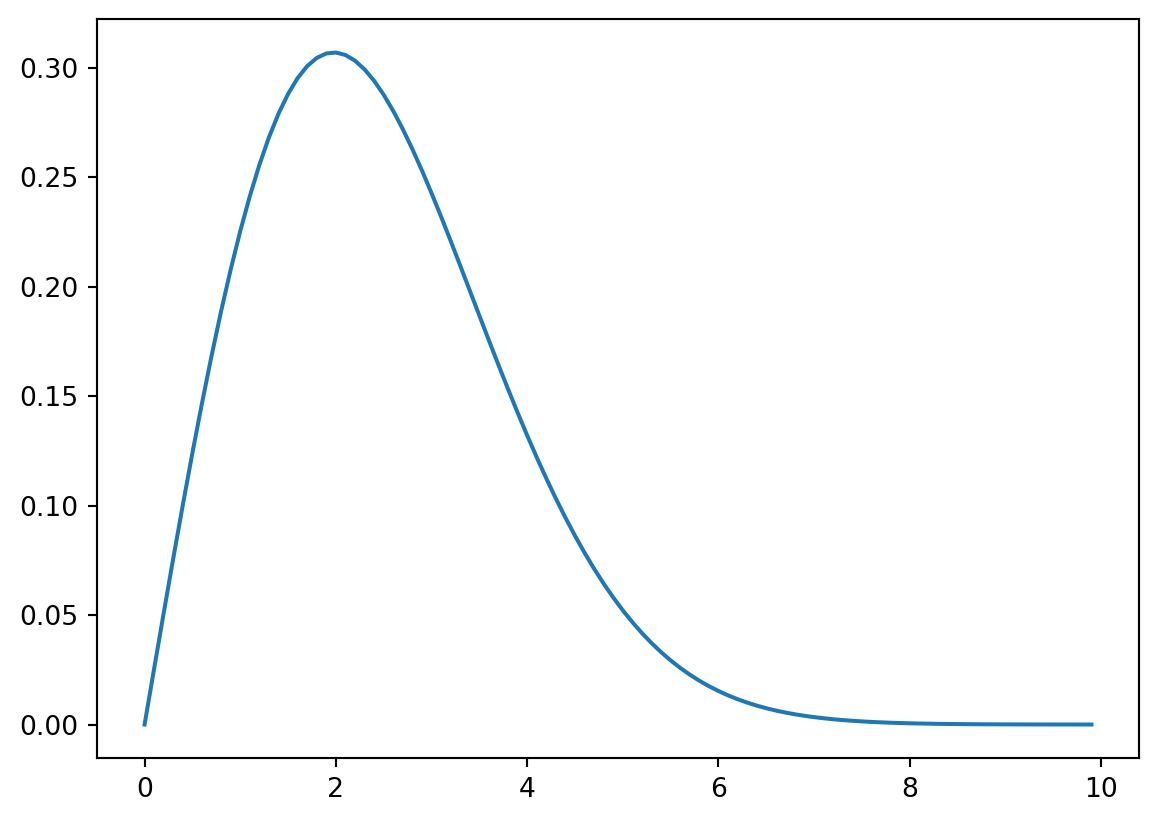
import scipy.stats as st
import matplotlib.pyplot as plt
import numpy as np
xx = np.arange(0,10,0.1)
zz = st.expon.pdf(xx,scale=3)
yy = st.weibull_min.pdf(xx, c = 2, scale = 3)
plt.close()
plt.plot(xx,zz, label = "Sensor A")
plt.plot(xx,yy, label = "Sensor B")
plt.xlabel("Failure time (years)")
plt.ylabel("Density")
plt.legend()

If \(A_F\) and \(B_F\) are the failure times of sensors \(A\) and \(B\), then the failure time of the entire system, denoted by \(S_F\) is

\[ S_F = \min\left(A_F, B_F\right) \]

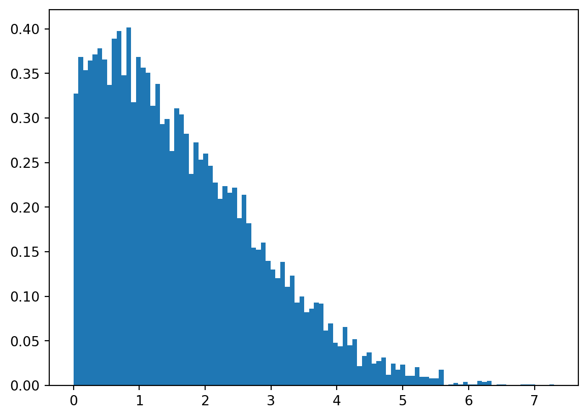
We can simulate the distrubtion of \(S_F\) and its properties like mean, median, and variance.

R = 10000
AF = st.expon.rvs(size=R,scale=3)
BF = st.weibull_min.rvs(size=R, c = 2, scale = 3)
SF = np.minimum(AF, BF)
plt.close()
plt.hist(SF, density = True,bins=100)
Summary = {
      "Mean":f"{SF.mean().item():.2f} (years)"
    , "Median":f"{np.median(SF).item():.2f} (years)"
    , "SD":f"{np.std(SF).item():.2f} (years)"
    , "Var":f"{np.var(SF).item():.2f} (years^2)"
}
import pandas as pd
sum1 = pd.DataFrame.from_dict(Summary, orient = "index", columns= ["Initial"])
sum1
Initial
Mean 1.64 (years)
Median 1.41 (years)
SD 1.19 (years)
Var 1.42 (years^2)

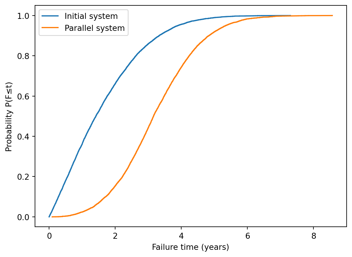
Consider an improvement of the system, in which additional sensors are added in parallel.

The new system fails either when all of the A sensors fail or when all of the B sensors fail. The failure time of the sensors are all independent.

(A) Using simulation, generate a density estimate of the failure time for the improved system using the histogram. (Compare it to the previous distribution by placing the histograms of the old and new systems in the same plot.)

(B) Add another column to the table of summary measures for the improved system.

R = 10000
AF = st.expon.rvs(size=(R,3),scale=3)
BF = st.weibull_min.rvs(size=(R,3), c = 2, scale = 3)
As = np.amax(AF,axis=1)
Bs = np.amax(BF,axis=1)
SF2 = np.minimum(As,Bs)
plt.close()
plt.hist(SF, bins = 100, density=True, color="#ff000050", label = "Initial system")
plt.hist(SF2, bins = 100, density=True, color="#0000ff50", label = "Parallel system")
plt.legend()
Summary2 = {
      "Mean":f"{SF2.mean().item():.2f} (years)"
    , "Median":f"{np.median(SF2).item():.2f} (years)"
    , "SD":f"{np.std(SF2).item():.2f} (years)"
    , "Var":f"{np.var(SF2).item():.2f} (years^2)"
}
sum1.assign(Parallel  = Summary2)
Initial Parallel
Mean 1.64 (years) 3.24 (years)
Median 1.41 (years) 3.16 (years)
SD 1.19 (years) 1.21 (years)
Var 1.42 (years^2) 1.48 (years^2)

(C) Create a single figure with the eCDF of both systems. Be sure to include a legend or labels.

from statsmodels.distributions.empirical_distribution import ECDF
f1 = ECDF(SF)
plt.close()
plt.step(f1.x, f1.y, where='post', label = "Initial system")
f2 = ECDF(SF2)
plt.step(f2.x, f2.y, where='post', label = "Parallel system")
plt.legend()
plt.xlabel("Failure time (years)")
plt.ylabel("Probability P(F≤t)")
Text(0, 0.5, 'Probability P(F≤t)')

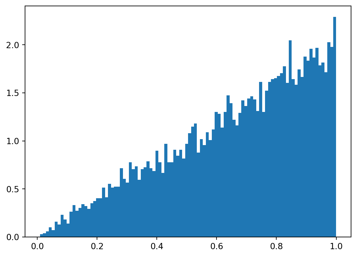
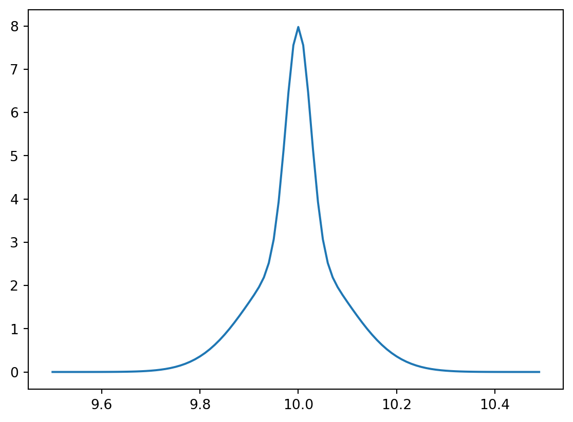
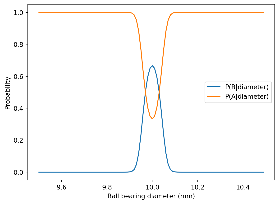
Q19 Ball bearings from machine A have diameters which follow a normal distribution with mean 10 and standard deviation 0.1. Machine B is more precise and generates ball bearings with the same mean but with a smaller standard deviation of 0.025. The additional precision comes at a cost: for every 1 ball bearing generated by machine B, machine A is able to produce 2 bearings.

(A) Generate a plot of the marginal density of ball bearing diameters generated at the factory. (The factory only has machines A and B.)

xx = np.arange(9.5,10.5,0.01)
ay = st.norm.pdf(xx, loc = 10, scale = 0.1)
by = st.norm.pdf(xx, loc = 10, scale = 0.025)
yy = 2/3*ay + 1/3*by
plt.close()
plt.plot(xx,yy)

(B) Calculate the probability that a randomly selected ball bearing came from machine B given that its diameter is 9.9.

bd = 1/3*by / (2/3*ay + 1/3*by)
ad = 2/3*ay / (2/3*ay + 1/3*by)
plt.close()
plt.plot(xx,bd, label = "P(B|diameter)")
plt.plot(xx,ad, label = "P(A|diameter)")
plt.legend()
plt.xlabel("Ball bearing diameter (mm)")
plt.ylabel("Probability")
Text(0, 0.5, 'Probability')

Q20 The Monte Hall problem is a classic game show. Contestants on the show where shown three doors. Behind one randomly selected door was a sportscar; behind the other doors were goats.

At the start of the game, contestants would select a door, say door A. Then, the host would open either door B or C to reveal a goat. At that point in the game, the host would ask the contestant if she would like to change her door selection. Once a contestant decided to stay or change, the host would open the chosen door to reveal the game prize, either a goat or a car.

Consider two strategies:

  1. Always stay with the first door selected.
  2. Always switch to the unopened door.

(A) Use simulation to determine the probability that each strategy wins the sportscar. The following code will simulate a single game. You may want to tweak it so that it generates results for R replicates.

R=10000
initial_choice = 1
car_door = np.random.randint(1, 3+1, size=R)
stay_win = 1*(car_door == initial_choice)
switch_win = []
for i in range(R):
    if car_door[i] == initial_choice:
        switch_win.append(0)
    else:
        switch_win.append(1*(np.random.randint(1, 3-1, size=1).item() == 1))
out = {"Stay":stay_win, "Switch":switch_win}

import pandas as pd
pd1 = pd.DataFrame(out)
pd.crosstab(pd1["Stay"], pd1["Switch"], normalize = True)
Switch 0 1
Stay
0 0.0000 0.6652
1 0.3348 0.0000

The “stay” strategy wins 1/3 of games. The “switch” strategy wins the remaining 2/3 or games. (Note, with 3 doors, one of the strategies must win each game.)

(B) Modify the code so that it works for a game with \(N\) doors. Calculate the probability of winning for each strategy with \(N=4\).

R=10000
N = 4
initial_choice = 1
car_door = np.random.randint(1, N+1, size=R)
stay_win = 1*(car_door == initial_choice)
switch_win = []
for i in range(R):
    if car_door[i] == initial_choice:
        switch_win.append(0)
    else:
        switch_win.append(1*(np.random.randint(1, N-1, size=1).item() == 1))
out = {"Stay":stay_win, "Switch":switch_win}

import pandas as pd
pd1 = pd.DataFrame(out)
pd.crosstab(pd1["Stay"], pd1["Switch"], normalize = True)
Switch 0 1
Stay
0 0.3699 0.3863
1 0.2438 0.0000

With 4 doors, the switch strategy is still better. (Note, with 4 doors, there are games when both strategies lose.)