
11 MLE
Recall that in this part of the text, we tackle the problem of constructing models (or updating beliefs) from data. Because data collection is also a source of uncertainty, we investigate how to appropariately propagate the uncertainty to the inferences (aka, answers to our questions) that we pulled from the models. Communicating the uncertainty associated with our answers will be key.
The goal of estimation is to find a probability model that describes the collected data so that, ultimately, we can answer questions about a larger population.
Note that there are several ways to use the data to estimate a probability model.
Options:
Eyeball
Today: ECDF Kernel density estimation (nonparametric)
Method of moments (parametric)
Today: Maximum likelihood (parametric)
Bayesian posterior (parametric)
11.1 Key question
\[ \text{Suppose } X \sim F_X \text{ where } F_X \text{ is unknown.}\\ \text{How might one estimate } F_X \text{ from } \underbrace{\boldsymbol{X}_N}_{\text{data}} ?\]
11.1.1 ECDF with Birthweight data
import numpy as np
birthweight = np.array([2523, 2551, 2557, 2594, 2600, 2622, 2637, 2637, 2663, 2665, 2722, 2733, 2751, 2750, 2769, 2769, 2778, 2782, 2807, 2821, 2835, 2835, 2836, 2863, 2877, 2877, 2906, 2920, 2920, 2920, 2920, 2948, 2948, 2977, 2977, 2977, 2977, 2922, 3005, 3033, 3042, 3062, 3062, 3062, 3062, 3062, 3080, 3090, 3090, 3090, 3100, 3104, 3132, 3147, 3175, 3175, 3203, 3203, 3203, 3225, 3225, 3232, 3232, 3234, 3260, 3274, 3274, 3303, 3317, 3317, 3317, 3321, 3331, 3374, 3374, 3402, 3416, 3430, 3444, 3459, 3460, 3473, 3544, 3487, 3544, 3572, 3572, 3586, 3600, 3614, 3614, 3629, 3629, 3637, 3643, 3651, 3651, 3651, 3651, 3699, 3728, 3756, 3770, 3770, 3770, 3790, 3799, 3827, 3856, 3860, 3860, 3884, 3884, 3912, 3940, 3941, 3941, 3969, 3983, 3997, 3997, 4054, 4054, 4111, 4153, 4167, 4174, 4238, 4593, 4990, 709, 1021, 1135, 1330, 1474, 1588, 1588, 1701, 1729, 1790, 1818, 1885, 1893, 1899, 1928, 1928, 1928, 1936, 1970, 2055, 2055, 2082, 2084, 2084, 2100, 2125, 2126, 2187, 2187, 2211, 2225, 2240, 2240, 2282, 2296, 2296, 2301, 2325, 2353, 2353, 2367, 2381, 2381, 2381, 2410, 2410, 2410, 2414, 2424, 2438, 2442, 2450, 2466, 2466, 2466, 2495, 2495, 2495, 2495])

import matplotlib.pyplot as plt
plt.hist(birthweight)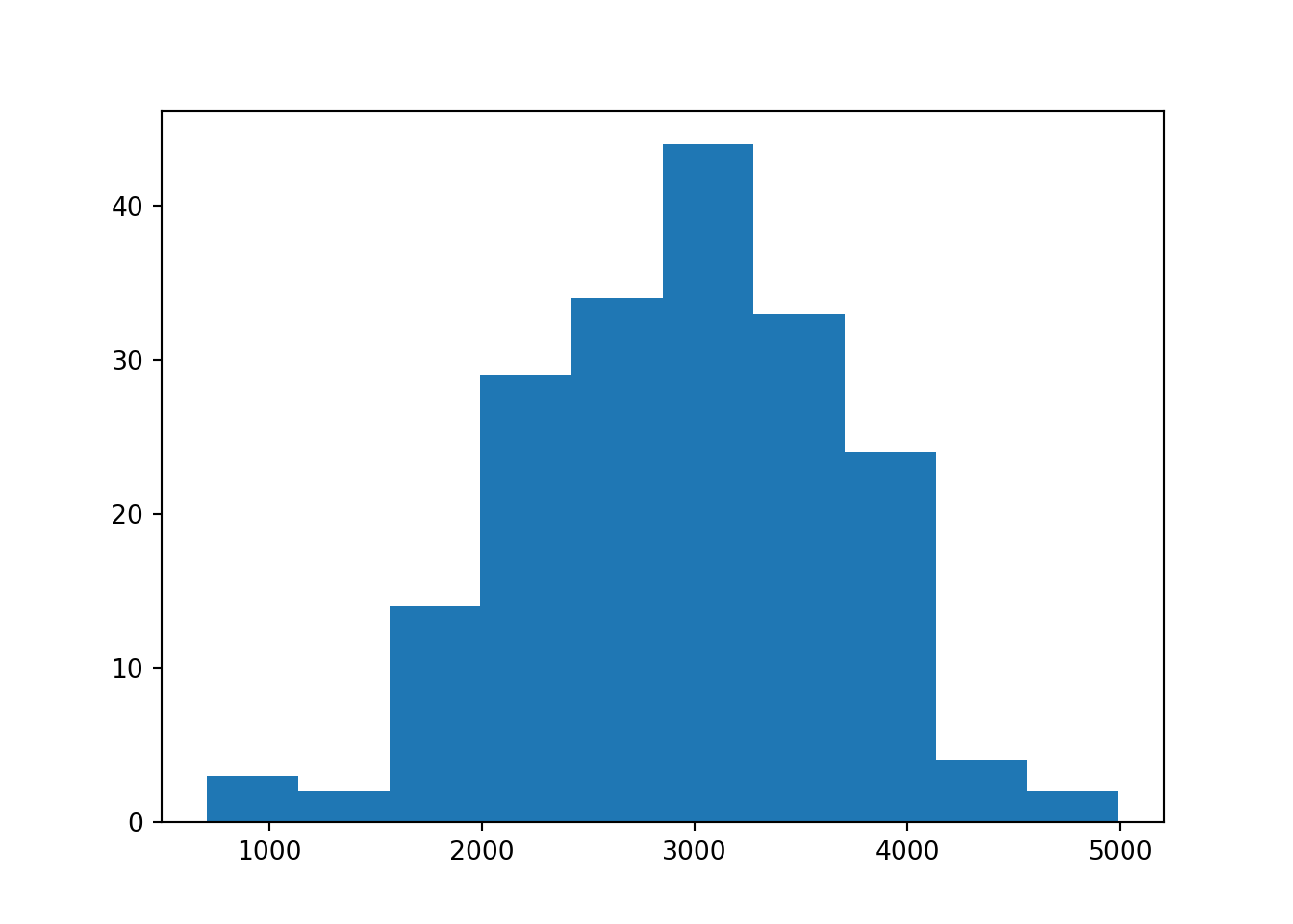
Empirical Cumulative Distribution Function as an estimate of the unknown CDF of a continuous random variable + Properties: + Like all CDFs, the eCDF takes candidate values as inputs and returns cumulative left hand probabilities as outputs. + The domain is the range of all possible candidate outcomes. + The range is 0 to 1. + The function is non-decreasing. + In Python, we can generate the eCDF, calculate estimated probabilities, and plot from it. + Drawbacks: + The eCDF is like stair steps. The function has abrupt jumps. + Often, the underlying distribution is believed to be smooth.
In the context of the birthweight data, we defined the eCDF in the following way: \[ \hat{F}(x) = \frac{\#\text{ birth weights} \leq x}{\#\text{ infants in dataset}} \] Let’s reexpress the eCDF. Let \(\text{bwt}_i\) denote the \(i^{th}\) birth weight in the data frame. Define \[ 1(\text{bwt}_i \leq x) = \left\{\begin{array}{ll}1 & \text{bwt}_i \leq x \\ 0 & \text{otherwise} \end{array} \right. \] This is often called the stair step function because of it’s shape. Here we use \(\text{bwt}_i=3000\) and plot the function.
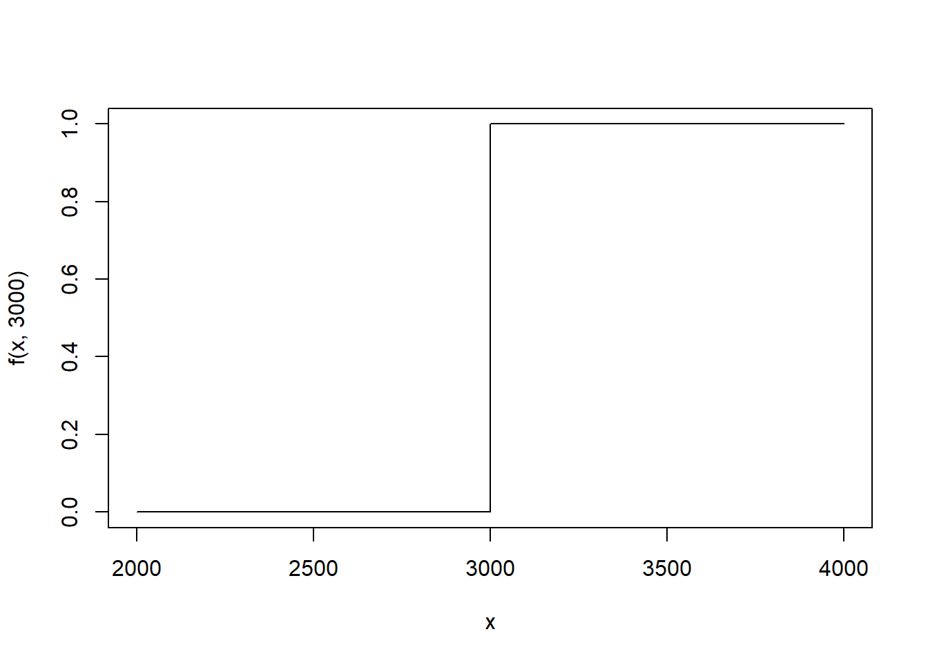
In words, stair step function is 1 when the \(i^{th}\) birth weight is less than \(x\) and 0 when it is more than \(x\). To calculate the number of observations in the data frame that have a birth weight less than \(x=2000\) grams, we can sum over every birth weight in the data frame. \[ \begin{aligned} \text{\# birth weights} \leq 2000 & = 1(\text{bwt}_1 \leq 2000) + 1(\text{bwt}_2 \leq 2000) + \dots + 1(\text{bwt}_n \leq 2000) \\ & = \sum_{i=1}^n 1(\text{bwt}_i \leq 2000) \end{aligned} \] To get the empirical proportion, we can divide by the number of observations in the data frame, typically denoted with \(n\) or \(N\).
In general, for any candidate birth weight, \(x\), the eCDF is \[ \hat{F}(x) = \sum_{i=1} \frac{1}{n} 1(\text{bwt}_i \leq x) \] Because \(1(\text{bwt}_i \leq x)\) is a stair-step, the eCDF is also stair-steppy, with abrupt jumps.
plt.close()
from statsmodels.distributions.empirical_distribution import ECDF
fhat = ECDF(birthweight)
plt.step(fhat.x, fhat.y, where='post')
plt.title(r'ECDF $\hat{F}_X$')
plt.xlabel('x')
plt.ylabel('Fn(x)')
plt.grid(True, alpha=0.3)
plt.show()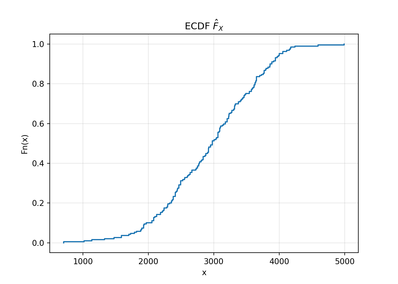
The ECDF is an important data visualization. It is a visualization of the CDF much like the histogram is a visualization of the PDF.
11.1.2 Maximum likelihood estimation
In this section, you will learn about maximum likelihood estimation (MLE) which is one way (not the only way) to estimate a smooth distribution (both CDF and PDF) from data.
MLE is a very commonly used method.
11.2 The big idea behind MLE
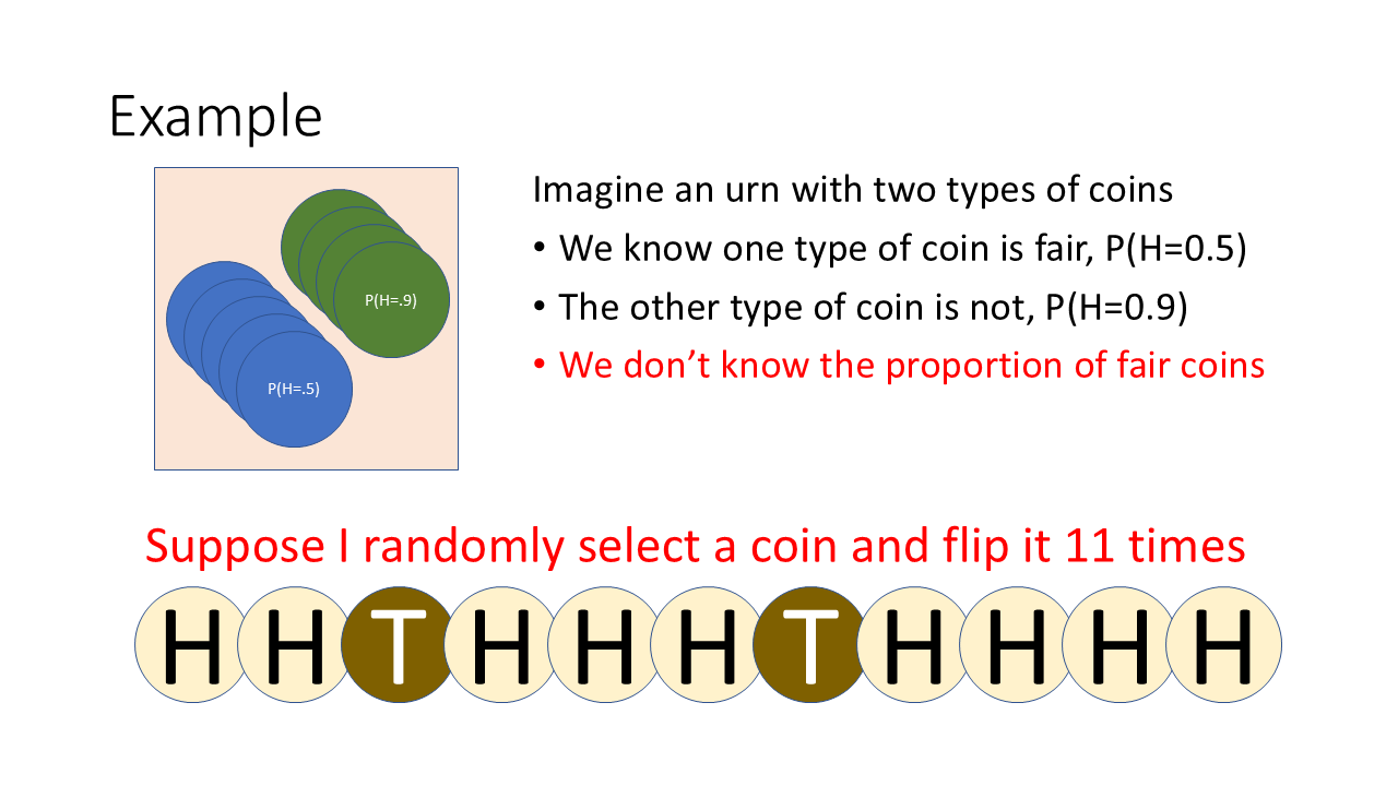

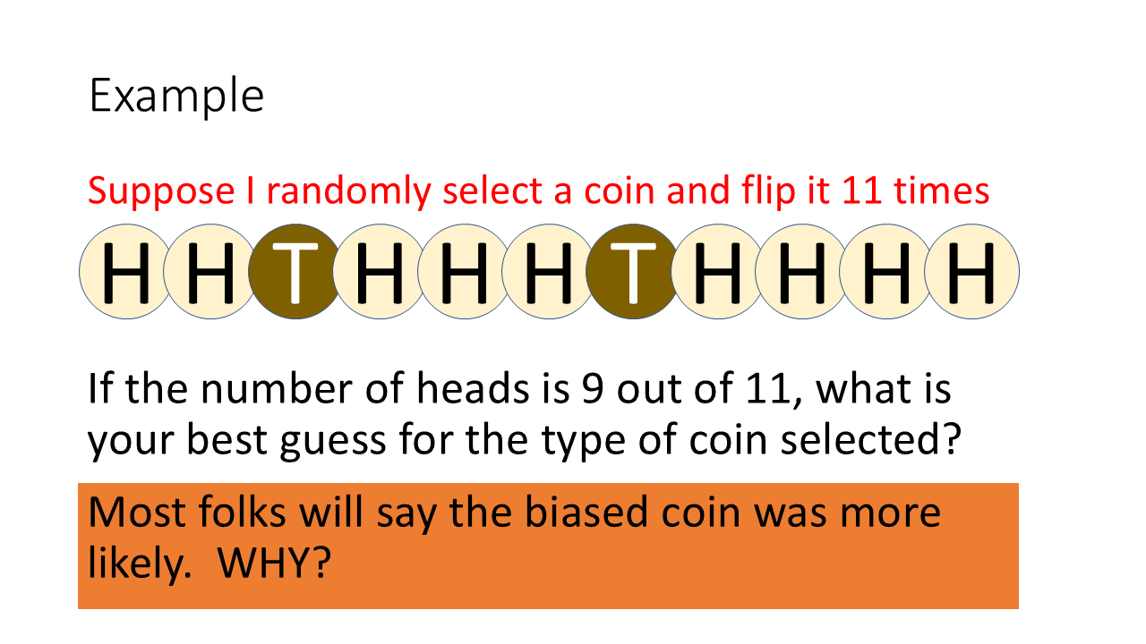
ANSWER: Maximum likelihood
11.3 Maximum Likelihood
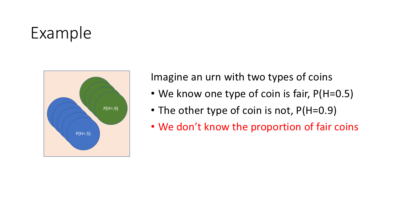
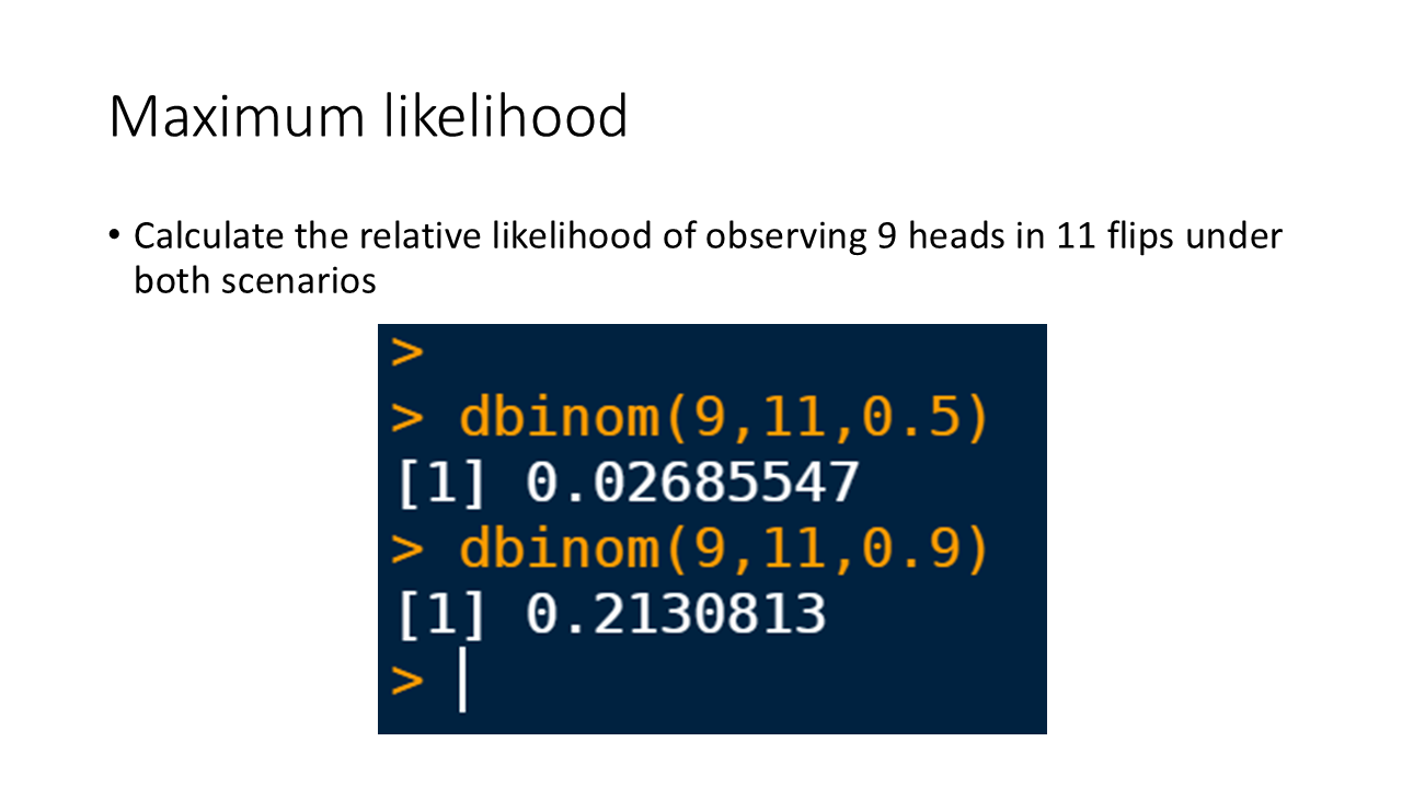
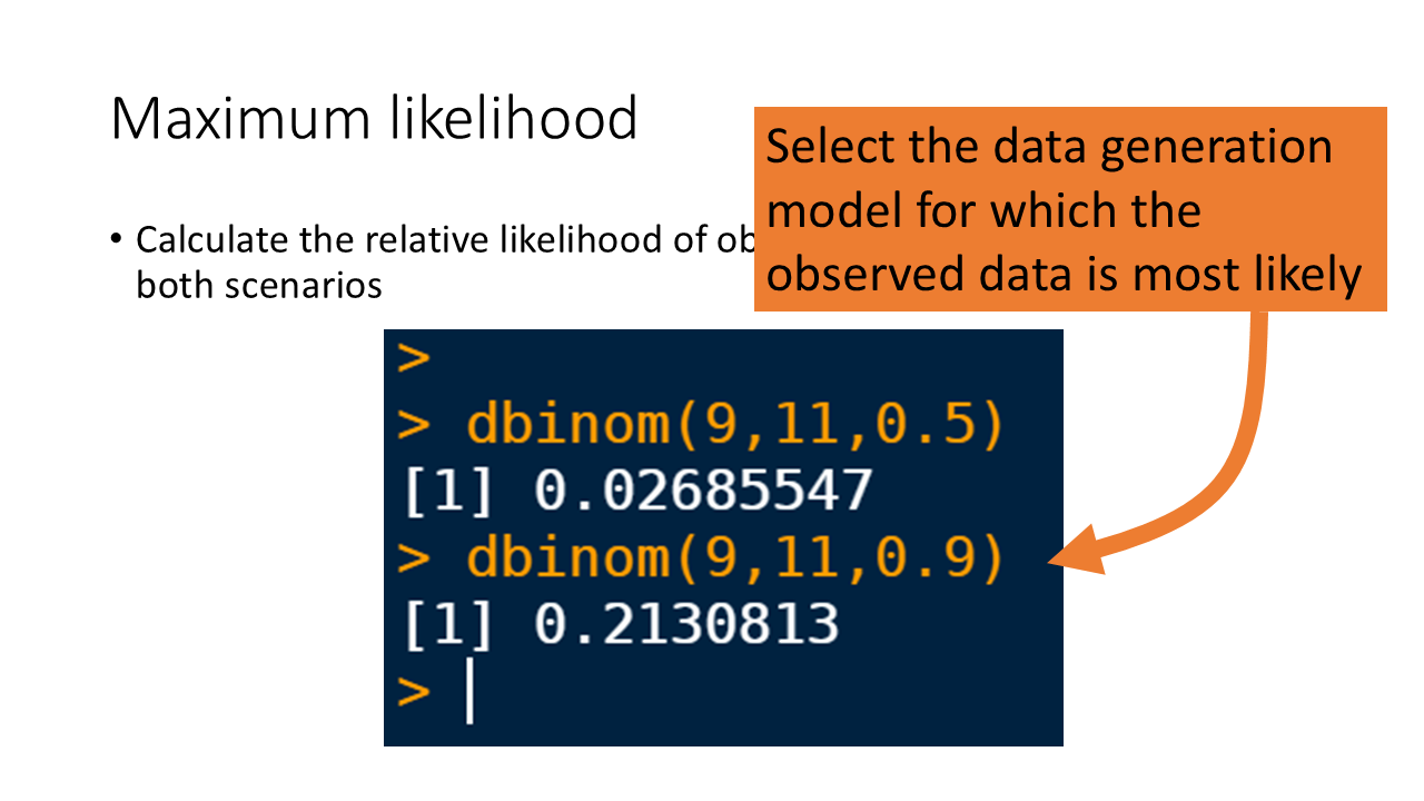
Calculate the relative likelihood of ovserving 9 heads in 11 flips under both scenarios.
from scipy.stats import binom
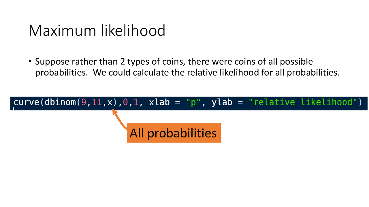
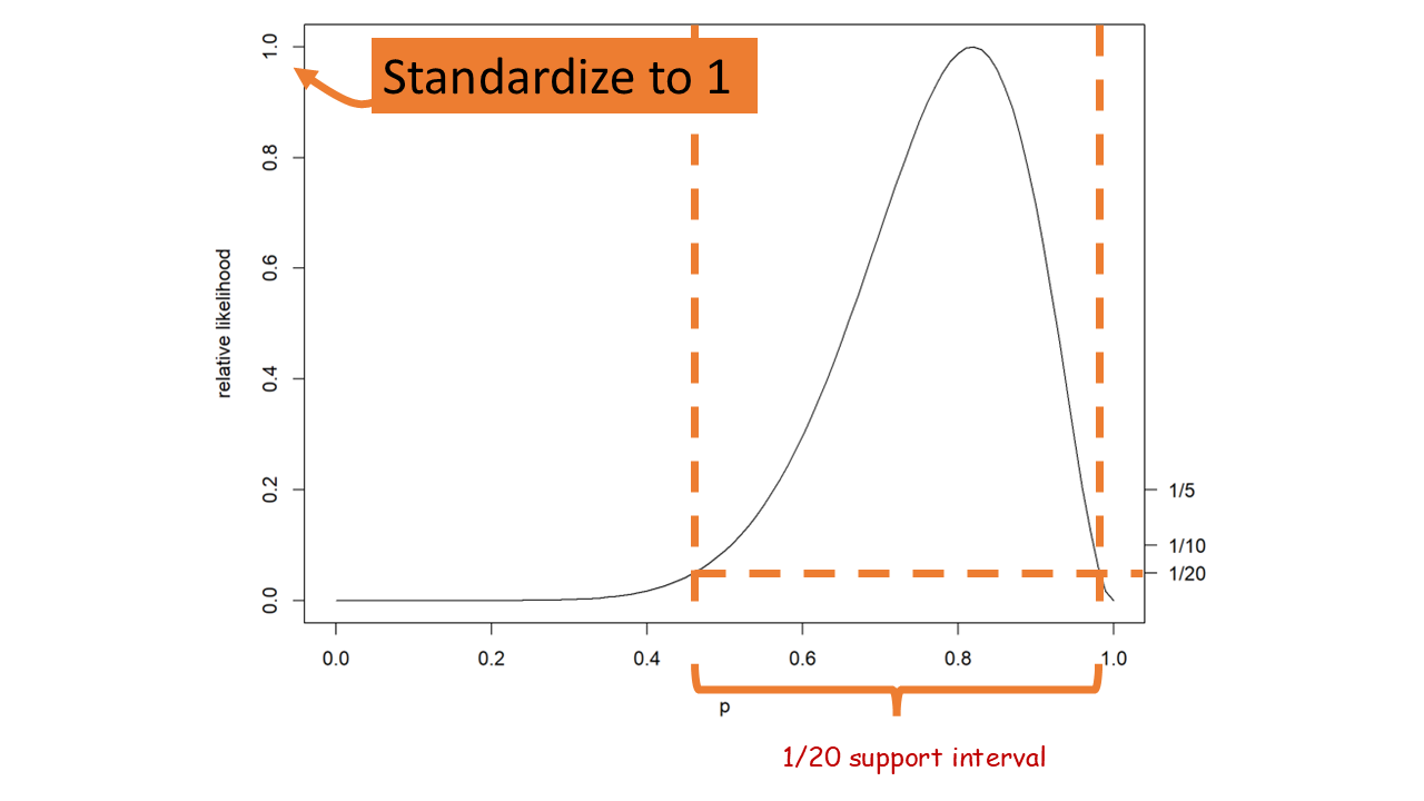
binom.pmf(9, 11, 0.5).item()0.026855468749999983binom.pmf(9, 11, 0.9).item()0.2130812689499999Suppose rather than 2 types of coins, there were coins of all possible probabilities. WE could calculate the relative likelihood for all probabilities.
x = np.linspace(0, 1, 1000)
y = binom.pmf(9, 11, x)

plt.plot(x, y)
plt.xlabel('p')
plt.ylabel('Relative Likelihood')
plt.grid(True, alpha=0.3)
plt.show()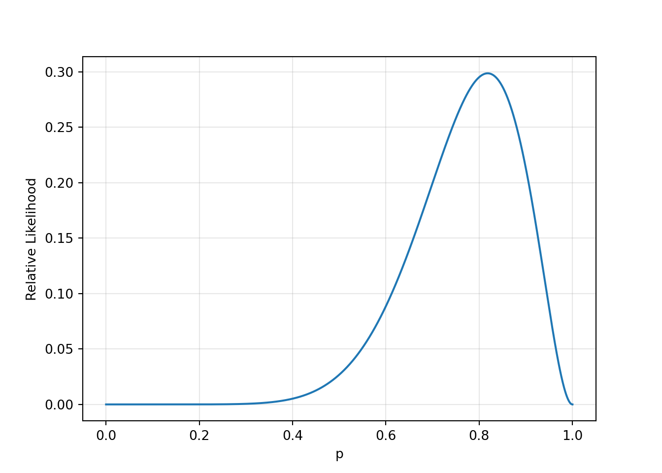
11.4 Maximum likelihood details
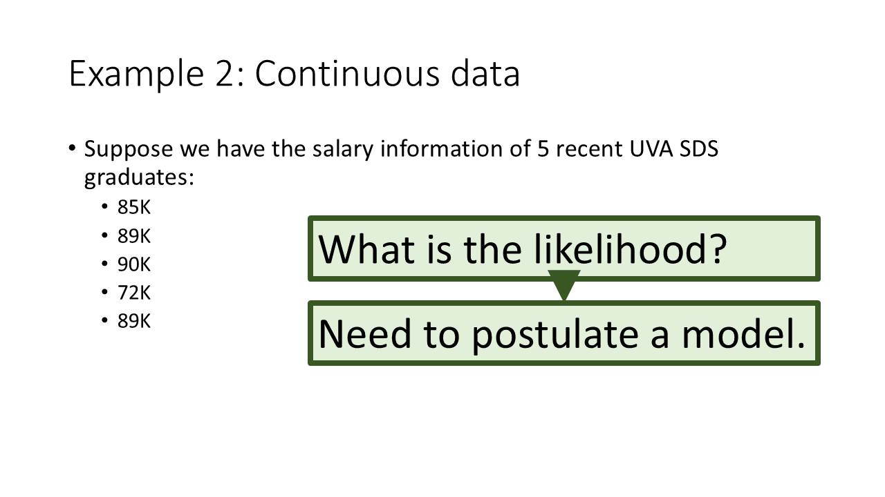
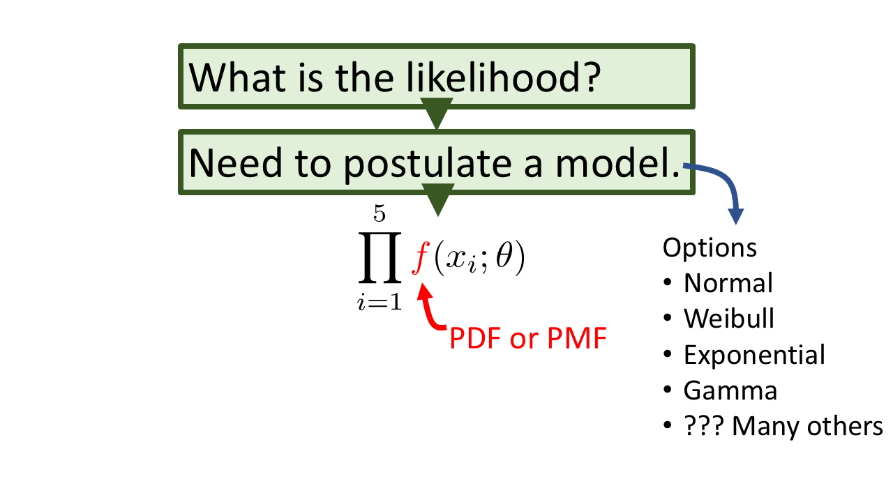
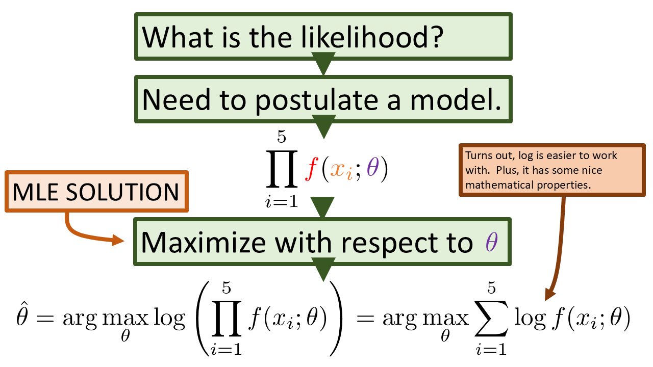
If the distribution of \(X\) is known, then \[ f_X(x |\ \theta) \] is the density function or the relative likelihood function for a single outcome.
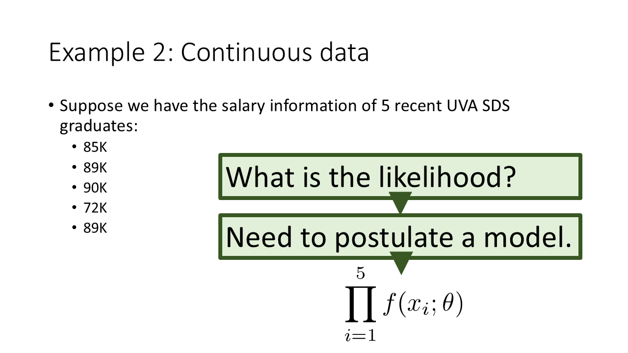
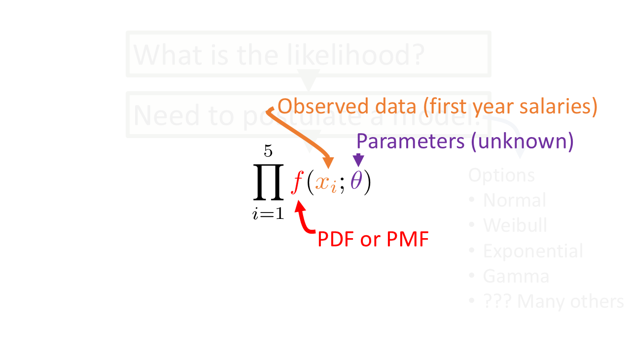
When the observations of the sample are independent, the density function for a sample, \(\boldsymbol{X}_N\) is \[f_{\boldsymbol{X}_N}(\boldsymbol{x}|\ \theta) = \prod_{i=1}^N f_X(x_i|\ \theta)\]
In the usual setting, \(\theta\) is known. Now suppose that \(\boldsymbol{x}\) is known.
\[L(\theta|\ \boldsymbol{x}) = f_{\boldsymbol{X}_N}(\boldsymbol{x}|\ \theta)\]
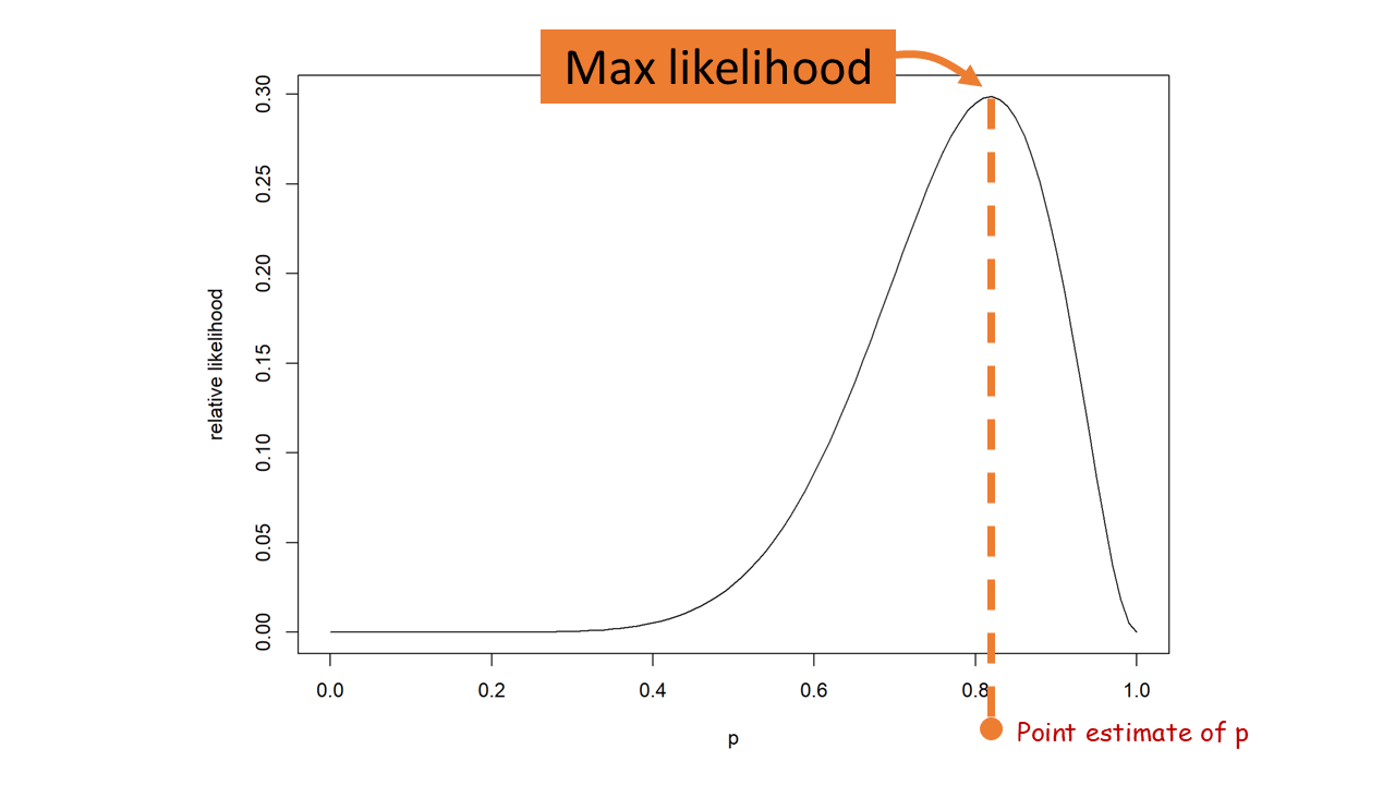
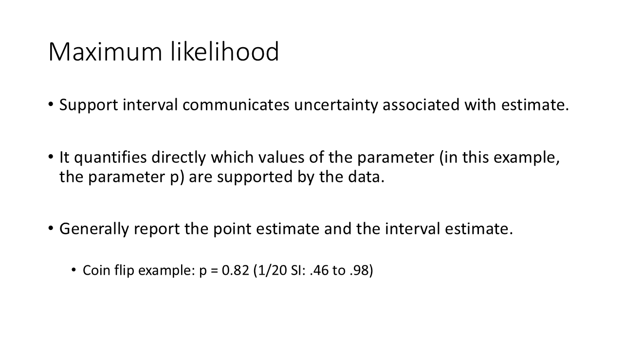
This is the likelihood function. The maximum likelihood solution is the parameter, \(\theta\), which maximizes the function. One can use visualization tools, mathematics (calculus or linear algebra), or computational optimization algorithms to find a solution.
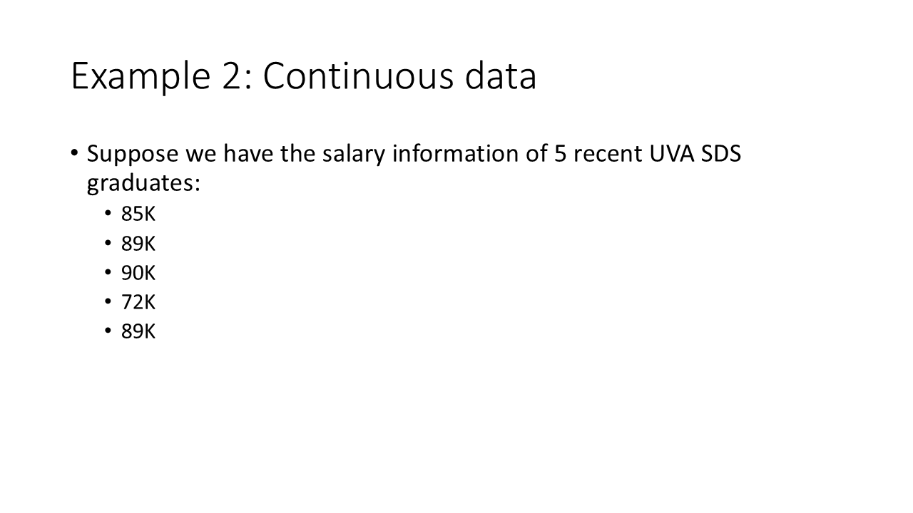
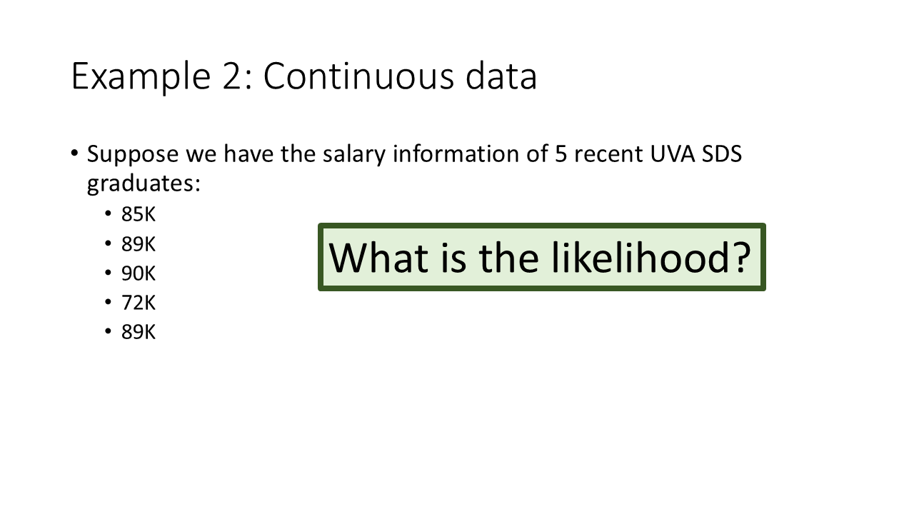
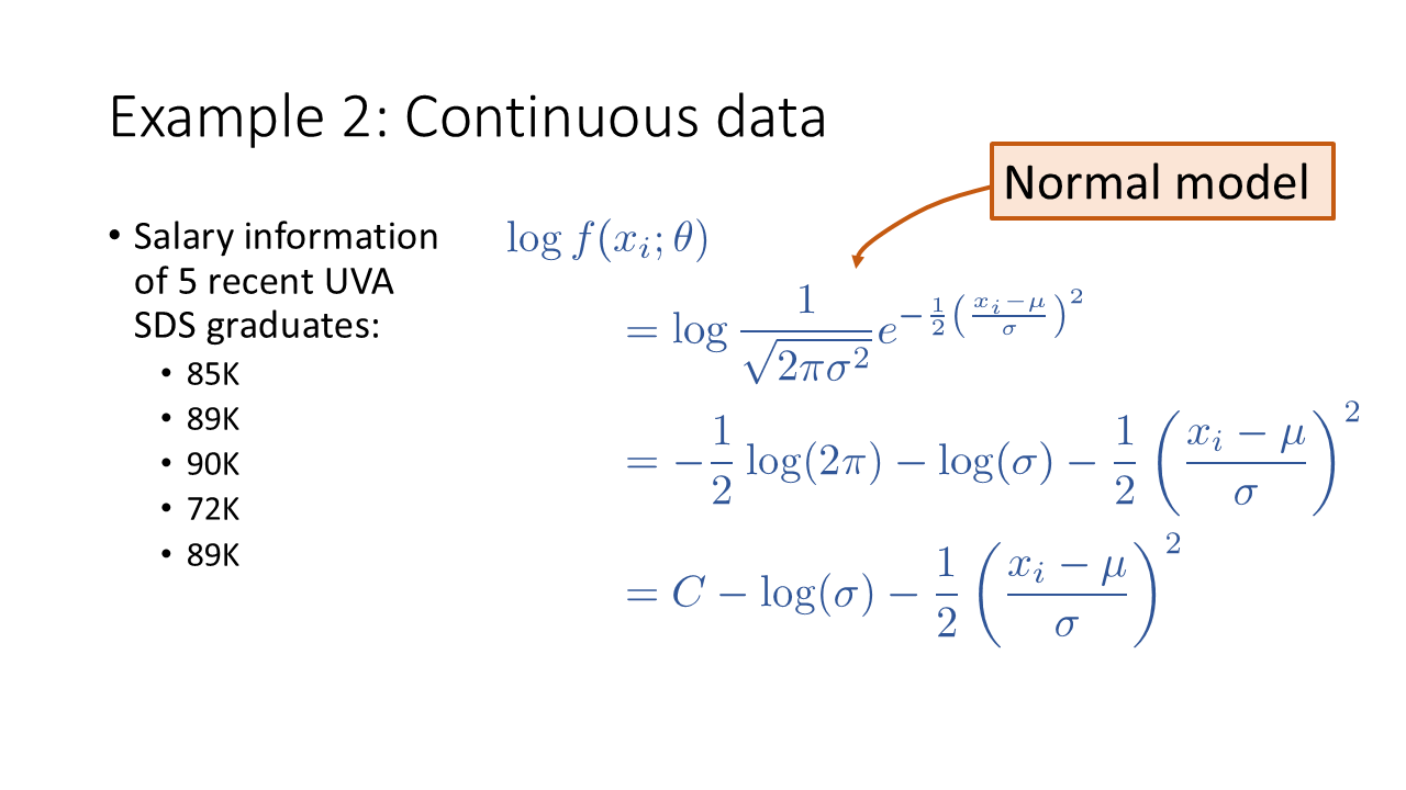
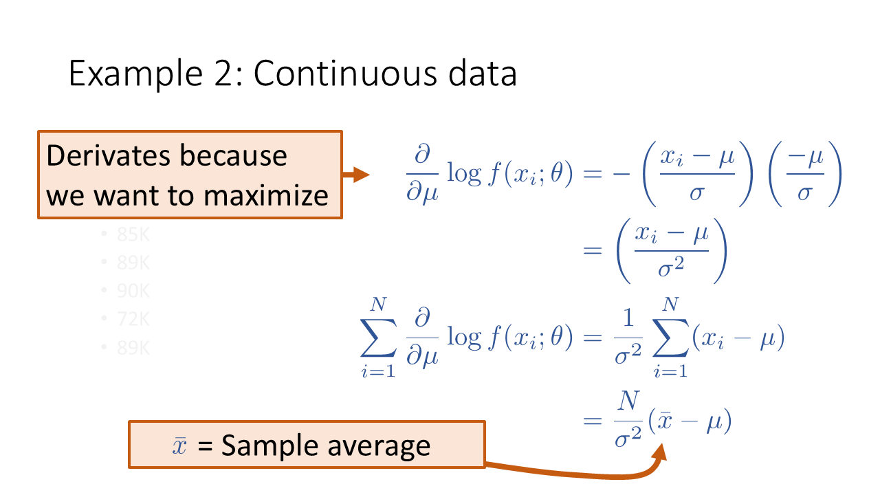
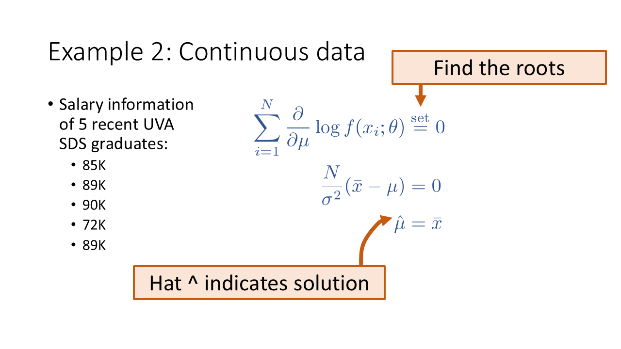
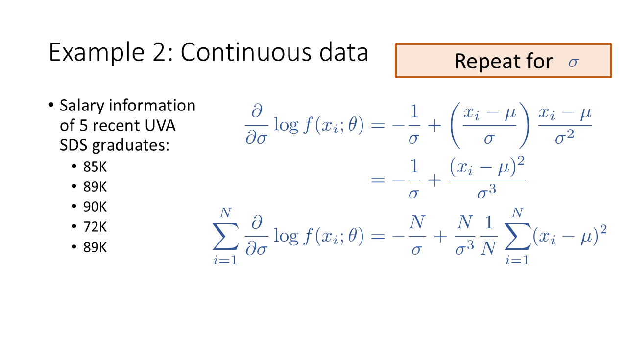
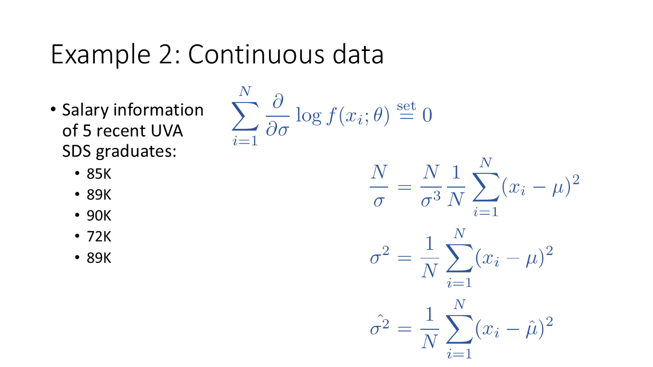
11.5 Example 2: Salary data
11.5.1 Example 4: BMI
Hmisc::getHdata(nhgh)
bmi <- nhgh$bmi
For the sake of discussion, suppose that scale is known to be 1.7. (We’ll get to the multivariable setting later.)
l <- function(shape, scale = 1.7, bmi){
  outer(shape, bmi, function(a,b)
    dgamma(
        x = b
      , shape = a
      , scale = 1.7
      , log = TRUE
    )
  ) %>% rowSums
}curve(l(x, 1.7, bmi), 0, 45, ylab = "", main = "log Likelihood", xlab = "shape")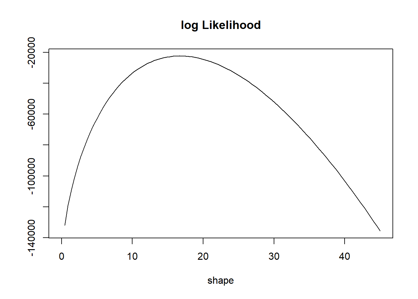
Note that the likelihood function is a function of the unknown parameter.
Strategy: Estimate the unknown parameter that maximizes the log likelihood.
Why does maximizing the likelihood make sense?
curve(l(x, 1.7, bmi), 0, 45, ylab = "", main = "log Likelihood", xlab = "shape")
xxx <- seq(15,22,by = 0.01)
# Poor mans maximization
mle <- l(xxx, 1.7, bmi) %>%
  which.max %>%
  `[`(xxx, .)
abline(v = mle, col = "blue", lwd = 3)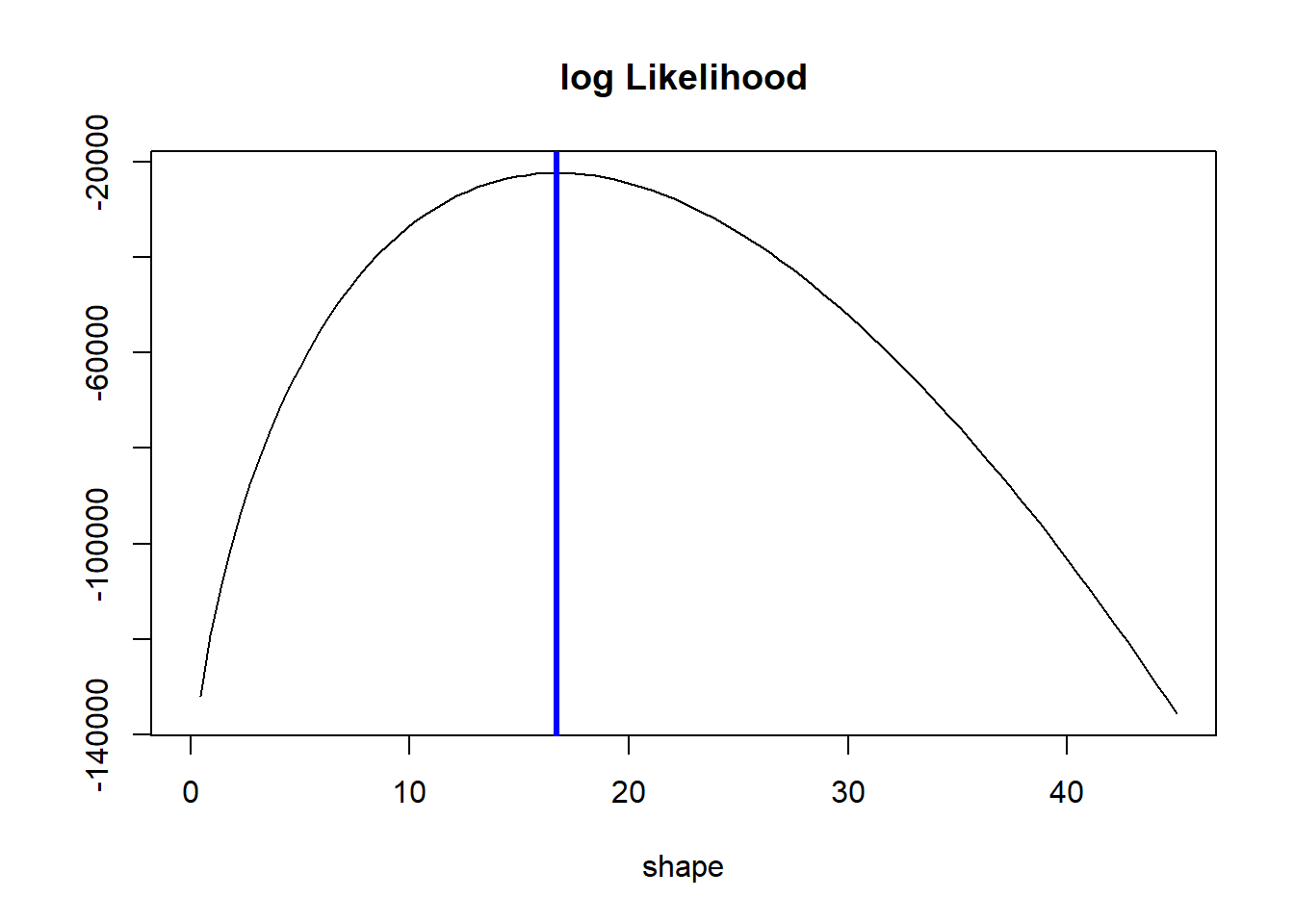
Will use the optim or optimize or mle function for maximization.
Now consider MLE with the normal distribution.
require(stats4)
nLL <- function(mean, sd){
  fs <- dnorm(
        x = bmi
      , mean = mean
      , sd = sd
      , log = TRUE
    )
  -sum(fs)
}
fit <- mle(
    nLL
  , start = list(mean = 1, sd = 1)
  , method = "L-BFGS-B"
  , lower = c(0, 0.01)
)
par(mfrow = c(1,2)); plot(profile(fit), absVal = FALSE)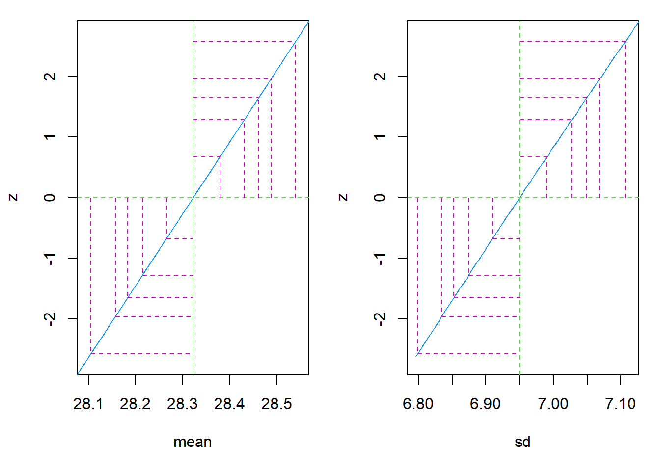
par(mfrow = c(1,2))
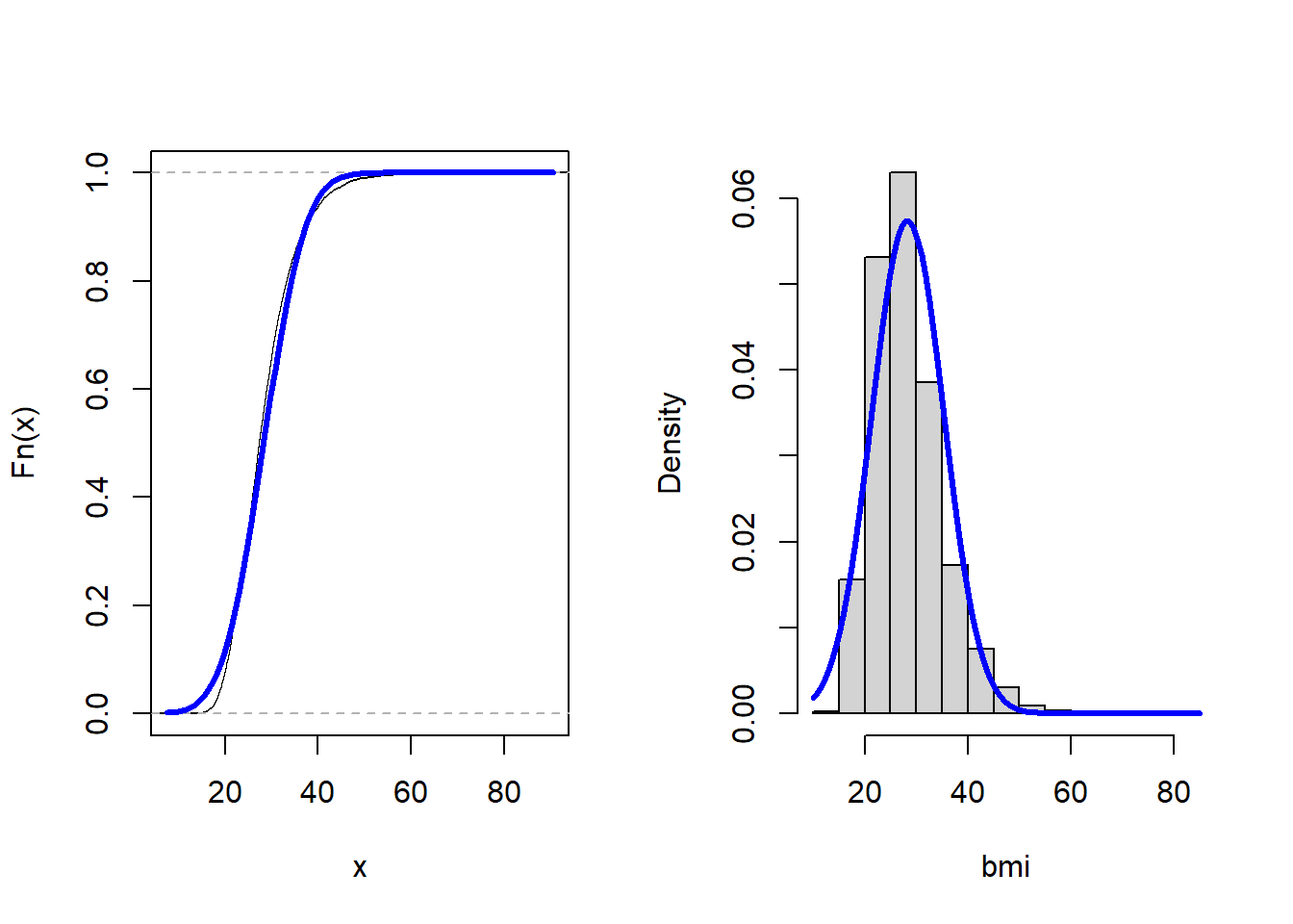
plot(ecdf(bmi), main = "")
curve(
pnorm(x, coef(fit)[1], coef(fit)[2])
, add = TRUE
, col = "blue"
, lwd = 3
)
hist(bmi, freq = FALSE, main = "")
curve(
dnorm(x, coef(fit)[1], coef(fit)[2])
, add = TRUE
, col = "blue"
, lwd = 3
)
Can use lm function to fit normal distribution, which is often easier.
lm(bmi ~ 1) %>% summary
Call:
lm(formula = bmi ~ 1)

Residuals:
Body Mass Index [kg/m^2s]
    Min      1Q  Median      3Q     Max
-15.142  -4.892  -1.032   3.558  56.548

Coefficients:
            Estimate Std. Error t value Pr(>|t|)
(Intercept) 28.32174    0.08431   335.9   <2e-16 ***
---
Signif. codes:  0 '***' 0.001 '**' 0.01 '*' 0.05 '.' 0.1 ' ' 1

Residual standard error: 6.95 on 6794 degrees of freedom
11.6 Hands-on
Estimate the distribution of arm length using the method of maximum likelihood. Generate plots of the estimated CDF and PDF.
Hmisc::getHdata(nhgh)