7 Combinatorics

Combinatorics is a branch of mathematics concerned with counting, arrangement, and combination. It forms the backbone of many crucial concepts in probability and statistics, especially those relevant to data science.

7.0.1 Importance of Combinatorics in Data Science

Combinatorics provides the tools to:

Calculate Probabilities: When dealing with equally likely outcomes, calculating probabilities involves counting favorable outcomes and dividing by the total number of outcomes. This applies to various scenarios in data science, such as analyzing random samples, simulations, and probabilistic models.
Analyze Algorithms and Data Structures: Understanding the efficiency of algorithms, especially for large datasets, requires analyzing their computational complexity, often based on counting the operations involved.
Develop Machine Learning Models: Many machine learning algorithms rely on combinatorial principles for tasks such as feature selection, model building, and optimization.

7.0.2 Formula for Probabilities with Equally Likely Outcomes

When all outcomes in a sample space have the same chance of happening, we can calculate the probability of an event using a simple formula:

\[ P(A) = \frac{\text{number of outcomes in } A}{\text{number of outcomes in the sample space } \Omega} = \frac{|A|}{|\Omega|} \]

Where:

$P(A)$ represents the probability of event A occurring.
$|A|$ is the number of outcomes where event A occurs.
$|\Omega|$ is the total number of outcomes in the sample space.

In simpler terms: To find the probability of something happening when all outcomes are equally likely, you count how many times that specific thing can happen and divide it by the total number of possibilities.

Example: Imagine you have a bag with 5 red marbles and 5 blue marbles. You want to find the probability of picking a red marble.

Event A: Picking a red marble
$|A|$ = 5 (There are 5 red marbles)
$|\Omega|$ = 10 (There are 10 total marbles)

Therefore, the probability of picking a red marble is: $P(A) = \frac{5}{10} = \frac{1}{2} = .5 = 50\%$

7.0.2.1 Factorials

The factorial of a non-negative integer n, denoted by n!, is the product of all positive integers less than or equal to n.

n! = 1 × 2 × 3 × … × (n - 1) × n

Special Case:

0! = 1

Examples:

5! = 1 × 2 × 3 × 4 × 5 = 120
3! = 1 × 2 × 3 = 6
1! = 1

Code in R:

You can calculate factorials in R using the factorial() function:

factorial(n)

For instance, factorial(5) would return 120.

7.1 Fundamental Principles of Counting

7.1.1 Multiplication Rule

If an operation can be done in $n_1$ ways and a second operation can be done in $n_2$ ways, then the two operations can be performed in $n_1 \cdot n_2$ ways. This rule can be extended to multiple operations.

7.1.1.1 Multiplication Rule Example: Choosing Outfits

Suppose you have 5 different shirts, 3 different pairs of pants, and 2 different pairs of shoes.

Question: You want to know how many different outfits you can create.

Solution using the Multiplication Rule:

Step 1: Choose a shirt. You have 5 options.
Step 2: Choose a pair of pants. You have 3 options.
Step 3: Choose a pair of shoes. You have 2 options.

Using the multiplication rule, you can calculate the total number of outfits:

Total Outfits = (Number of shirt choices) * (Number of pant choices) * (Number of shoe choices) = 5 * 3 * 2 = 30

Therefore, you can create 30 different outfits.

7.1.2 The Inclusion-Exclusion Principle

The inclusion-exclusion principle is a counting technique used to determine the size of a union of multiple sets. It is particularly helpful when the sets overlap, as simply adding the sizes of the individual sets would lead to overcounting.

Basic Idea

To find the size of the union of two sets, A and B, we:

Include: Add the sizes of the individual sets: |A| + |B|.
Exclude: Subtract the size of their intersection to correct for overcounting: |A ∩ B|.

This gives the formula: |A ∪ B| = |A| + |B| - |A ∩ B|

Extending to Multiple Sets

The principle can be extended to more than two sets. For three sets A, B, and C, the formula becomes:

|A ∪ B ∪ C| = |A| + |B| + |C| - |A ∩ B| - |A ∩ C| - |B ∩ C| + |A ∩ B ∩ C|

Notice the alternating pattern of adding and subtracting intersections of increasing size.

7.1.2.1 Example: Counting Students Taking Multiple Courses

Suppose 100 students are enrolled in at least one of three courses: Algebra (A), Calculus (C), and Statistics (S). We are given the following information about the number of students in each course and their intersections:

|A| = 50
|C| = 40
|S| = 30
|A ∩ C| = 20
|A ∩ S| = 15
|C ∩ S| = 10
|A ∩ C ∩ S| = 5

Question: How many students are taking at least one of these courses?

Solution using the Inclusion-Exclusion Principle:

We want to find |A ∪ C ∪ S|. Applying the formula for three sets:

|A ∪ C ∪ S| = |A| + |B| + |C| - |A ∩ B| - |A ∩ C| - |B ∩ C| + |A ∩ B ∩ C|

Substituting the given values:

|A ∪ C ∪ S| = 50 + 40 + 30 - 20 - 15 - 10 + 5 = 80

Therefore, 80 students are taking at least one of the three courses.

Explanation:

Inclusion: We start by adding the number of students in each individual course: 50 + 40 + 30.
Exclusion: Since some students are taking more than one course, we have overcounted them. We subtract the number of students in each pair-wise intersection: -20 - 15 - 10.
Inclusion: We have now undercounted the students taking all three courses because they were added three times initially, then subtracted three times. We add back the number of students in the intersection of all three sets: +5.

This process ensures that each student is counted exactly once, resulting in the accurate total number of students taking at least one of the courses.

7.2 Permutations

Permutations deal with the arrangement of objects in a specific order.

Permutations without replacement involve arranging distinct objects where repetition is not allowed.

Example. Permutations without replacement of 4 letters (A,B,C,D) taken 3 at the time:

Counting sequences without replacement

The number of permutations without replacement of 4 distinct objects taken 3 at a time is

\[ P_{3,4} = 4 \cdot (4-1) \cdot (4-2) = 4 \cdot 3 \cdot 2 = 24 \]

In general, the number of permutations without replacement of n distinct objects taken k at a time is \[ P_{k,n} = n \cdot(n-1) \cdot (n-2) \dots (n-k+1) = \dfrac{n!}{(n-k)!} \].

7.2.1 Example: Assigning Graders to Exam Questions

A professor has 10 teaching assistants (TAs) and wants to assign a different TA to grade each of the 4 questions on an exam. The order in which the TAs are assigned to questions matters because each question has a different level of difficulty.

Step 1: Choose a TA for the first question. There are 10 options.
Step 2: Choose a TA for the second question. With one TA already assigned, there are 9 options left.
Step 3: Choose a TA for the third question. There are 8 remaining TAs to choose from.
Step 4: Choose a TA for the fourth question. There are 7 TAs remaining.

To find the total number of possible assignments, we use the multiplication rule: 10 * 9 * 8 * 7 = 5040

This calculation demonstrates the principle of permutations without replacement. Once a TA is assigned to a question, they are not available for other questions, and the specific question they grade matters in the overall assignment scheme.

We get to the same result by applying the formula

\[ P_{k, n} = \dfrac{n!}{(n - k)!} \]

Where:

n is the total number of distinct objects in the group.
k is the size of the subset being selected.

In this example:

n = 10 (the number of TAs)
k = 4 (the number of exam questions)

Thus

\[ P_{4, 10} = \dfrac{10!}{(10 - 4)!} = \dfrac{10!}{6!} = 10 * 9 * 8 * 7 = 5040 \]

This result confirms the calculation obtained using the multiplication rule.

7.2.2 Example: Recommender Systems and Permutation Without Replacement.

Imagine a music streaming service with a vast catalog of 1 million songs. The service wants to create a personalized 10-song playlist for a user. We’ll demonstrate how the concept of permutation without replacement applies to this scenario.

Step 1: Choosing the First Song: The system has 1,000,000 options for the first song in the playlist. It can choose any song from the entire music library.
Step 2: Choosing the Second Song: Once the first song is selected, the system can’t recommend the same song again. This means there are only 999,999 songs left to choose from for the second slot in the playlist.
Step 3: Choosing the Third Song: With two songs already in the playlist, the system has 999,998 options remaining for the third song.
Continuing the Process: This pattern continues for each subsequent song selection. The number of available choices decreases by one with each step, as repetition is not allowed.
Step 10: Choosing the Tenth Song: By the time the system reaches the tenth song, there are 999,991 songs remaining to choose from.

To calculate the total number of possible 10-song playlists, we multiply the number of choices at each step:

1,000,000 * 999,999 * 999,998 * … * 999,991

This massive number represents the total possible permutations without replacement for creating a 10-song playlist from a library of 1 million songs.

This step-by-step breakdown illustrates how the concept of permutation without replacement is relevant in data science, particularly in recommender systems. The order of songs in a playlist matters for the listener’s experience, and the system cannot recommend the same song multiple times within the same playlist. This aligns with the conditions for permutations without replacement: order is significant, and repetition is not allowed.

Permutations with replacement involve arranging objects when repetition is allowed.

Example. Permutations with replacement of 4 letters (A,B,C,D) taken 3 at the time:

The number of permutations of 4 objects taken 3 at a time with replacement is $4 \cdot 4 \cdot 4 = 4^3$.

In general, the number of permutations of N objects taken k at a time with replacement is

\[N^k\].

7.2.3 Example. Permutations with Replacement: PIN Codes

A four-digit PIN code for a bank card can use any digit from 0 to 9 for each of the four positions.

There are 10 choices for the first digit.
There are 10 choices for the second digit.
There are 10 choices for the third digit.
There are 10 choices for the fourth digit.

This means that the total number of possible four-digit PIN codes is: 10 * 10 * 10 * 10 = 10,000.

Explanation:

Replacement: In this scenario, replacement is allowed because you can repeat digits within the PIN. For example, “1111” is a valid PIN.
Order Matters: The order of the digits is crucial. The PIN “1234” is different from “4321”. This is why we use permutations, as they account for the order of elements.

7.3 Combinations

Combinations deal with the selection of objects where order does not matter. The number of combinations of n distinct objects taken k at a time (“n choose k”) is
\[ C_{k,n} = \dfrac{n!}{k!(n-k)!} = \binom{n}{k} \] You can calculate combinations in R using the choose(n,k) function. For instance:

7.3.1 Combinations as Permutations Divided by Permutations

The formula for combinations (ways to choose items from a set without regard to order) can be understood as a division of permutations. It’s derived by dividing the number of permutations (arrangements where order matters) by the number of permutations possible within each combination.

Explanation:

Start with Permutations: The number of ways to arrange k items chosen from a set of n, where order does matter (permutations), is given by:

\[P_{k, n} = \dfrac{n!}{(n - k)!}\]

Permutations Within a Combination: Consider a specific combination of k items. These k items can be arranged in k! different ways, representing k! different permutations of that same combination.
Removing Order: To find the number of combinations, we essentially need to eliminate the effect of order within each group of k items. We achieve this by dividing the total number of permutations by the number of permutations possible for each combination. This leads to the formula for combinations:

\[C_{k, n} = \dfrac{P_{k, n}}{k!} = \dfrac{n!}{k!(n - k)!}\]

In other words, the formula for combinations is a result of dividing the number of permutations (where order matters) by the number of permutations possible within each combination (to remove the effect of order). This division ensures that we count each unique combination only once, regardless of how the elements within it are arranged.

7.3.2 Example:

Let’s say we have a set of three letters: {A, B, C}. We want to find the number of ways to choose 2 letters from this set, without regard to order.

Permutations (Order Matters): The permutations of size 2 from this set are: AB, BA, AC, CA, BC, CB. There are 6 permutations.
Combinations (Order Doesn’t Matter): The combinations of size 2 are: AB, AC, BC. Notice that BA is considered the same combination as AB, and so on. There are only 3 unique combinations.

The formula reflects this process:

$C_{2, 3} = \dfrac{P_{2, 3}}{2!} = \dfrac{3!}{2!(3 - 2)!} = 3$

We divided the 6 permutations by 2! (the number of ways to arrange 2 items), effectively collapsing permutations like AB and BA into a single combination.

7.3.3 Example: Market Basket Analysis

Consider a grocery store wanting to perform market basket analysis to understand customer purchasing patterns. The store has data on 1000 different products, and they want to analyze which combinations of 3 products are frequently purchased together.

Order Doesn’t Matter: In market basket analysis, the order of products in a basket is not significant. A basket containing milk, bread, and eggs is the same as a basket with eggs, milk, and bread.
No Repetition: We are interested in analyzing combinations of distinct products. Buying two cartons of milk wouldn’t be considered a combination of two different products.

To determine the number of possible combinations of 3 products that customers can purchase, we use the combinations formula. We have 1000 products (n = 1000) and we want to choose combinations of 3 (k = 3).

The number of combinations is calculated as:

$C_{3, 1000} = \dfrac{1000!}{3!(1000 - 3)!} = \dfrac{1000 * 999 * 998}{3 * 2} = 166,167,000$

Connection to Data Science:

This example shows the extensive number of possible product combinations even in a store with a relatively limited number of products. In data science, we use algorithms and techniques to handle this combinatorial complexity. Methods such as:

Association Rule Mining: To identify frequent itemsets (combinations of items) and generate rules like “If a customer buys X, they are likely to buy Y.”
Apriori Algorithm: An efficient way to discover frequent itemsets by exploiting the property that subsets of frequent itemsets must also be frequent.

7.3.4 Example: Recommender Systems

Consider a music streaming service with a library of 50,000 songs. The service wants to recommend personalized playlists of 10 songs to its users. To create these playlists, the service needs to analyze different combinations of 10 songs from its library.

Order Doesn’t Matter: The order of songs in a playlist doesn’t fundamentally change the playlist’s content. A playlist with songs A, B, and C is essentially the same as a playlist with songs C, A, and B.
No Repetition: Recommending the same song multiple times within a 10-song playlist would not be a good user experience.

The number of possible 10-song playlists from a library of 50,000 songs can be calculated using the combinations formula:

$C_{10, 50000} = \dfrac{50000!}{10!(50000 - 10)!}$

This results in an extremely large number of possible combinations.

Connection to Data Science:

Recommender systems use algorithms like collaborative filtering and content-based filtering to make personalized recommendations. These algorithms don’t need to evaluate every single combination of songs. Instead, they leverage user data and song characteristics to identify patterns and preferences, allowing them to efficiently generate relevant recommendations.

7.3.5 Example: Feature Selection in Machine Learning

Imagine a scenario where a machine learning model is being built to predict customer churn for a telecommunications company. There are 5 potential features that could be used in the model:

Monthly bill amount
Number of customer service calls
Data usage
Contract length
Age of the customer

To simplify the model and improve its interpretability, the team decides to select only 3 of these features to include. The order in which the features are selected doesn’t affect the model’s outcome. A model using features 1, 2, and 3 is the same as a model using features 3, 1, and 2.

To determine the number of possible combinations of 3 features from a set of 5, we can use the combinations formula:

$C_{3, 5} = \dfrac{5!}{3!(5-3)!} = \dfrac{5 * 4 * 3}{3 * 2} = 10$

Therefore, there are 10 different combinations of features that could be used in the model.

Connection to Data Science:

In practice, data scientists employ techniques like feature importance scores and recursive feature elimination to systematically select the most relevant features for a machine learning model. Combinations provide a theoretical foundation for understanding the number of possible feature subsets, while these techniques guide the selection process.

7.3.6 Practice Examples

Example 1: Probability of a Specific Poker Hand:

7.3.6.1 Question:

In a standard 52-card deck, what is the probability of getting a full house (3 cards of one rank and 2 cards of another)?

7.3.6.2 Solution:

We can use combinations to solve this. * First, choose one rank out of 13: $\binom{13}{1}$. * Choose 3 cards of that rank: $\binom{4}{3}$. * Choose a different rank: $\binom{12}{1}$. * Choose 2 cards of that rank: $\binom{4}{2}$. * The total number of full house hands is $\binom{13}{1}\binom{4}{3}\binom{12}{1}\binom{4}{2}$. * The total number of 5-card hands is $\binom{52}{5}$. * The probability of getting a full house is: $\dfrac{\binom{13}{1}\binom{4}{3}\binom{12}{1}\binom{4}{2}}{\binom{52}{5}}$.

Example 2: Random Sampling: You are analyzing a dataset of 1000 customer reviews, and you want to randomly select 50 reviews for a manual quality check.

7.3.6.2.1 Question: How many different samples of size 50 are possible?

7.3.6.2.2 Solution:

This is a combination without replacement because you don’t want to select the same review twice. The number of possible samples is $\binom{1000}{50}$.

Example 3: Building a Diverse Team

A data science company wants to form a team of 4 data scientists from a pool of 8 candidates. They are committed to building a diverse team and want to ensure that the team includes at least one man and one woman. Out of the 8 candidates, 5 are women and 3 are men.

7.3.6.2.3 Question:

How many different ways are there to form a 4-person team that includes at least one man and one woman?

7.3.6.2.4 Solution:

This problem can be solved using the concept of combinations and the principle of inclusion-exclusion.

Total Possible Teams: The total number of ways to choose a 4-person team from 8 candidates is given by the combination formula (Equation 5.4 from source):
${8 \choose 4} = \dfrac{8!}{4!4!} = 70$
Teams with All Women: The number of ways to choose a team of 4 women from the 5 female candidates is: ${5 \choose 4} = \dfrac{5!}{4!1!} = 5$
Teams with All Men: The number of ways to choose a team of 4 men from the 3 male candidates is: ${3 \choose 4} = 0$ (This is 0 because we cannot choose 4 men from a pool of only 3).
Teams with at Least One Man and One Woman: To get the number of teams with at least one man and one woman, we subtract the number of teams with all women and the number of teams with all men from the total number of possible teams:

$70 - 5 - 0 = 65$

Therefore, there are 65 ways to form a 4-person team that includes at least one man and one woman.

Example 4: Password Security

An online platform requires users to create passwords that are at least 6 characters long and must contain at least one lowercase letter, one uppercase letter, and one digit.

7.3.6.2.5 Question:

How many possible 6-character passwords meet these criteria?

7.3.6.2.6 Solution:

This problem can be solved using the product rule for k-tuples.

Total Possible Passwords: If there are no restrictions, each of the 6 characters in the password can be chosen from 26 lowercase letters, 26 uppercase letters, and 10 digits, giving a total of 62 possible choices per character. The total number of possible 6-character passwords without any restrictions is 62^6.
Passwords Not Meeting the Criteria: To find the number of passwords that meet the criteria, we can use a strategy similar to the inclusion-exclusion principle:
- Calculate the number of passwords that do not contain a lowercase letter (only uppercase letters and digits allowed: 36^6).
- Calculate the number of passwords that do not contain an uppercase letter (26 lowercase letters and 10 digits allowed: 36^6).
- Calculate the number of passwords that do not contain a digit (only lowercase and uppercase letters allowed: 52^6).
Passwords Meeting the Criteria: Subtract the number of passwords not meeting the criteria from the total number of possible passwords to get the number of passwords that meet the criteria.

The final answer is: 62^6 - 36^6 - 36^6 - 52^6.

7.3.6.2.7 Explanation:

This solution uses the idea of counting undesirable outcomes and subtracting them from the total possible outcomes to find the number of desirable outcomes. This strategy can be helpful when directly counting the desirable outcomes is more complex.

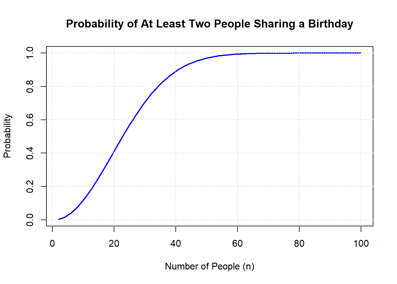
7.3.6.3 Example: The Birthday Problem

7.3.6.3.1 Question

The Birthday Problem is a famous problem in probability theory. It asks: What is the probability that in a group of ( n ) people, at least two people share the same birthday?

7.3.6.3.2 Solution

To solve this problem, we use the principle of complementary counting. Instead of directly calculating the probability that at least two people share the same birthday, we first calculate the probability that no one shares a birthday, and then subtract this from 1.

7.3.6.3.3 Step-by-Step Explanation

Assumptions:
- There are 365 days in a year (ignoring leap years).
- Each person’s birthday is equally likely to be any of the 365 days.
Calculate the probability that no two people share a birthday:
- For the first person, there are 365 possible days for their birthday.
- For the second person, there are 364 possible days (since they must have a different birthday from the first person).
- For the third person, there are 363 possible days, and so on.
The probability that all ( n ) people have different birthdays is: \[ P(\text{no shared birthdays}) = \frac{365}{365} \times \frac{364}{365} \times \frac{363}{365} \times \cdots \times \frac{365-n+1}{365} \]
Simplify the expression:
- This can be written as: \[ P(\text{no shared birthdays}) = \frac{365!}{(365-n)! \cdot 365^n} \]
- This is also the same as:

\[ P(\text{no shared birthdays}) = \frac{\text{Permutations \textbf{without} replacement of 365 days taken $n$ at the time}}{\text{Permutation \textbf{with} replacement of 365 days taken $n$ at the time}} = \frac{P_{n,365}}{365^n} \]

Calculate the probability that at least two people share a birthday:

The probability that at least two people share a birthday is the complement of the probability that no one shares a birthday: \[ P(\text{at least one shared birthday}) = 1 - P(\text{no shared birthdays}) \]

7.3.6.3.4 Example Calculation

Let’s calculate the probability for ( n = 23 ):

\[ P(\text{no shared birthdays}) = \frac{365}{365} \times \frac{364}{365} \times \frac{363}{365} \times \cdots \times \frac{343}{365} \approx 0.4927 \] Then \[ P(\text{at least one shared birthday}) = 1 - 0.4927 \approx 0.5073 \]

Thus, in a group of 23 people, there is approximately a 50.73% chance that at least two people share the same birthday.

7.3.6.3.5 Conclusion

The Birthday Problem illustrates how counterintuitive probability can be. Even with a relatively small group of 23 people, the probability of shared birthdays is surprisingly high, demonstrating the power of combinatorial counting and complementary probability.

7.3.6.4 R code

7.3.7 Practice Problems

Problem 1: Lottery Problem: A lottery requires players to choose 6 numbers from 1 to 49. What is the probability of winning the jackpot by matching all 6 numbers?

Problem 2: Committee Formation: A club has 12 members. How many ways can a committee of 4 members be formed?

Problem 3: Suppose you are building a machine learning model to predict customer churn. You have 10 features to choose from.

1. If you want to experiment with models using all possible combinations of 3 features, how many models do you need to build?
1. If computational constraints limit you to building models with at most 5 features, how many models can you build?

Problem 4: In a dataset of 10,000 emails, 1000 are spam. You randomly select 100 emails.

1. What is the probability that exactly 10 of the selected emails are spam?
1. What is the probability that at least one of the selected emails is spam?

These problems illustrate how combinatorics can be applied to various data science problems, providing insights and solutions.

Problem 5: [Analyzing Customer Reviews] A data science team is building a sentiment analysis model to classify customer reviews as positive, negative, or neutral. They have a dataset of 10,000 reviews, and they want to manually label a subset of 100 reviews for training the model. Due to time constraints, they decide to focus on labeling reviews that express strong sentiment (either highly positive or highly negative). They estimate that 20% of the reviews express strong positive sentiment, and 10% express strong negative sentiment.

How many different ways are there to choose 100 reviews for manual labeling if they don’t consider the sentiment of the reviews?
How many ways are there to choose 50 strongly positive reviews and 50 strongly negative reviews for labeling?