d1 <- MASS::birthwt
bwt <- d1$bwt
ecdf(bwt)(2500) # estimated probability that birth weight is less than or equal to 2500 grams
[1] 0.3121693plot(ecdf(bwt),do.points = FALSE, xlab = "Birth weight (grams)")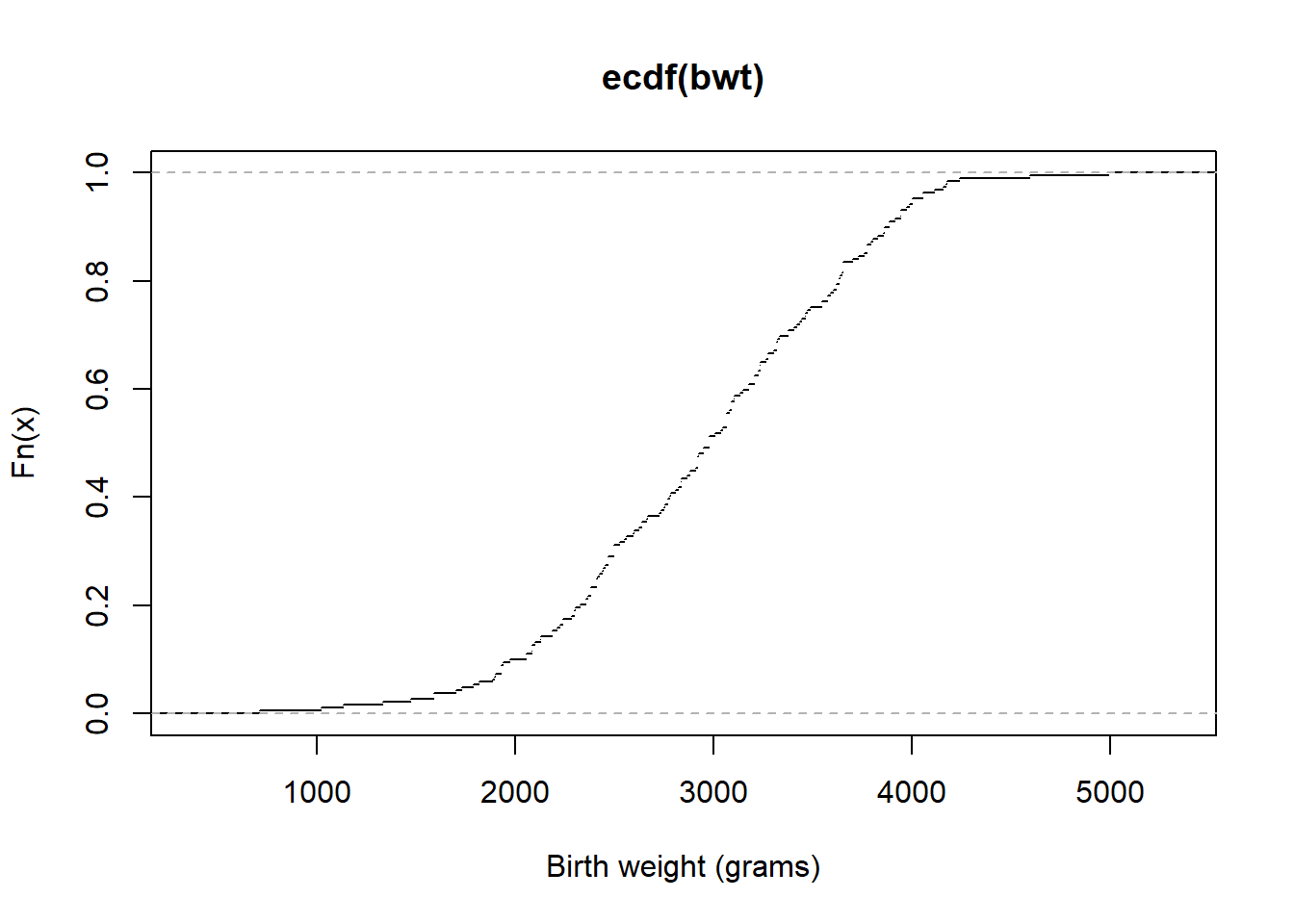
In the previous module, we learned about the
d1 <- MASS::birthwt
bwt <- d1$bwt
ecdf(bwt)(2500) # estimated probability that birth weight is less than or equal to 2500 grams[1] 0.3121693plot(ecdf(bwt),do.points = FALSE, xlab = "Birth weight (grams)")
Let’s return briefly to previous module. In the previous module, we considered the birth weight data. We defined the eCDF in the following way: \[ \hat{F}(x) = \frac{\#\text{ birth weights} \leq x}{\#\text{ infants in dataset}} \] Let’s reexpress the eCDF. Let \(\text{bwt}_i\) denote the \(i^{th}\) birth weight in the data frame. Define \[ 1(\text{bwt}_i \leq x) = \left\{\begin{array}{ll}1 & \text{bwt}_i \leq x \\ 0 & \text{otherwise} \end{array} \right. \] This is often called the stair step function because of it’s shape. Here we use \(\text{bwt}_i=3000\) and plot the function.
f <- function(x,bwt) 1*(bwt <= x)
curve(f(x, 3000),2000,4000,n=5000)  #If birth weight = 3000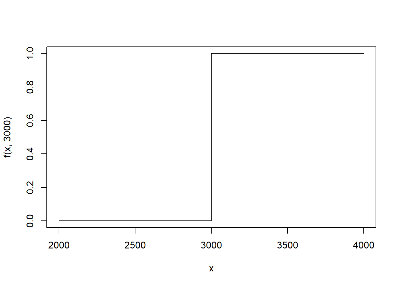
In words, stair step function is 1 when the \(i^{th}\) birth weight is less than \(x\) and 0 when it is more than \(x\). To calculate the number of observations in the data frame that have a birth weight less than \(x=2000\) grams, we can sum over every birth weight in the data frame. \[ \begin{aligned} \text{\# birth weights} \leq 2000 & = 1(\text{bwt}_1 \leq 2000) + 1(\text{bwt}_2 \leq 2000) + \dots + 1(\text{bwt}_n \leq 2000) \\ & = \sum_{i=1}^n 1(\text{bwt}_i \leq 2000) \end{aligned} \] To get the empirical proportion, we can divide by the number of observations in the data frame, typically denoted with \(n\) or \(N\).
In general, for any candidate birth weight, \(x\), the eCDF is \[ \hat{F}(x) = \sum_{i=1} \frac{1}{n} 1(\text{bwt}_i \leq x) \] Because \(1(\text{bwt}_i \leq x)\) is a stair-step, the eCDF is also stair-steppy, with abrupt jumps.
One strategy for creating a smooth estimate of the CDF is to replace the stair step function with a smooth alternative. There are lots of options. (See here (link).)
For example, consider replacing the stair step function with the Gaussian CDF centered at \(\text{bwt}_i\).
f <- function(x,bwt) 1*(bwt <= x)
curve(f(x, 3000),2000,4000,n=5000)  #If birth weight = 3000
g <- function(x,bwt,s) pnorm(x,bwt,s)
curve(g(x, 3000, 100), add=TRUE, lwd = 5, col = "red")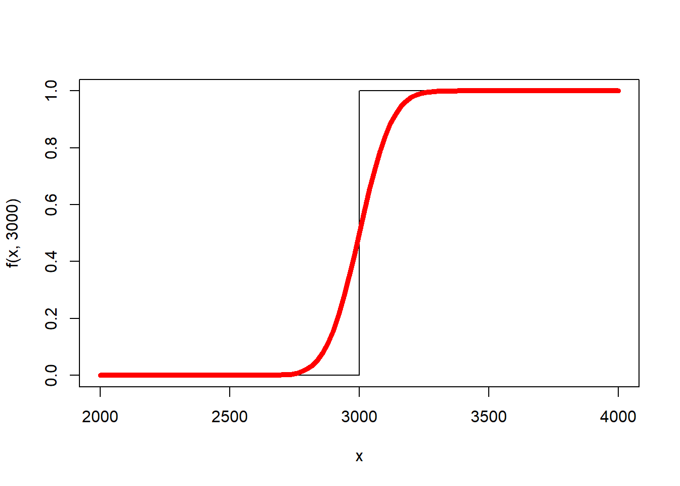
The resulting estimate of the distribution function is \[ \hat{F}(x) = \sum_{i=1} \frac{1}{n} \Phi(x,\text{bwt}_i, s) \]
Fhat <- function(x,s) rowMeans(outer(x,bwt,function(a,b) pnorm(a,b,s)))
plot(ecdf(bwt),do.points = FALSE)
curve(Fhat(x,100),add=TRUE,col="red",lwd=3)
legend("left", legend = c("eCDF","Gaussian"), col = c("black","red"), lwd = 3, bty = "n")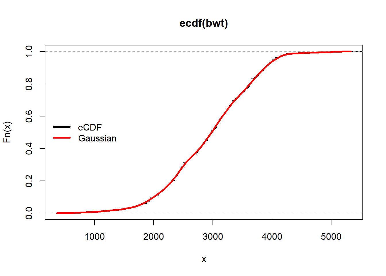
The degree of smoothing is controlled by the parameter s. We can increase or decrease the degree of smoothing by increasing or decreasing s.
plot(ecdf(bwt),do.points = FALSE)
curve(Fhat(x,100),add=TRUE,col="red",lwd=3)
curve(Fhat(x,300),add=TRUE,col="green",lwd=3)
legend("left", legend = c("eCDF","Gaussian (s=100)","Gaussian (s=300)"), col = c("black","red","green"), lwd = 3, bty = "n")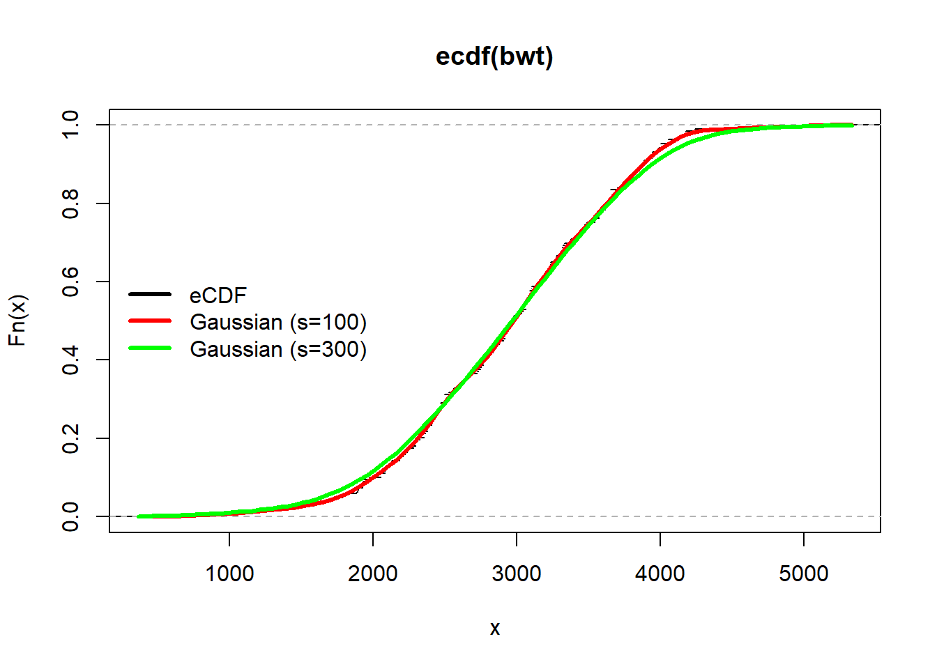
This type of estimation is known as kernel smoothing or kernel density estimation. The kernel refers to the specific function selected to replace the stair step function.
In the interactive calculator, your will explore 6 different kernels. Navigate to Birthweight KCDF (link).
In the calculator, you will see the standard eCDF (in black) and the stair step function (in red). A representative kernel function is shown for bwt=3000. As you click on different kernels, you’ll see how the estimate of distribution function changes. You’ll also see how kernel function changes. Also note how the kernels and resulting estimates of the distribution function change as s, the smoothing parameter, changes.
Assessment
s that generates a good estimate of the distribution function. Create an image of the estimated CDF for each kernel. (You can hide the representative kernel function by clicking the circle in line 15 of the calculator.)s were better or worse?age. Create a plot in which the eCDF of age is overlaid with the smooth kernel estimate.Call back: What is a PDF? What are the inputs? What are the outputs? Can you give an example of a PDF? What is the connection between a CDF and a PDF? (Can you verbalize your answers?)
We continue with the birth weight data, considering the PDF in addition to the CDF.
In a previous module, you “fit-by-eye” a normal, gamma, and mixture of two normals model. You are going to revisit that same data again, this time choosing the parameters while looking at both the resulting CDF and PDF.
Navigate here (link). Note: Typically CDFs and PDFs are on very different scales. The y-axis for a CDF goes from 0 to 1. The y-axis for a PDF can go from 0 to infinity. So that the CDF and PDF can be viewed on the same scale, the CDF has been multiplied by 0.001.
Hands on
In the previous module, you “fit-by-eye” the distribution of birth weight by overlaying the kernel estimate of \(\hat{F}\) to the eCDF. In this module we are going to look at both the kernel estimate of the CDF and the PDF. First, let’s derive the PDF of the kernel estimate.
Recall that the PDF is the derivative of the CDF (if the derivative exists). Using the usual notation of capital letters for CDFs and lower case letters for PDFs, let \(F\) denote the CDF of the random variable. Then \[ f(x) = \frac{dF(x)}{dx} \]
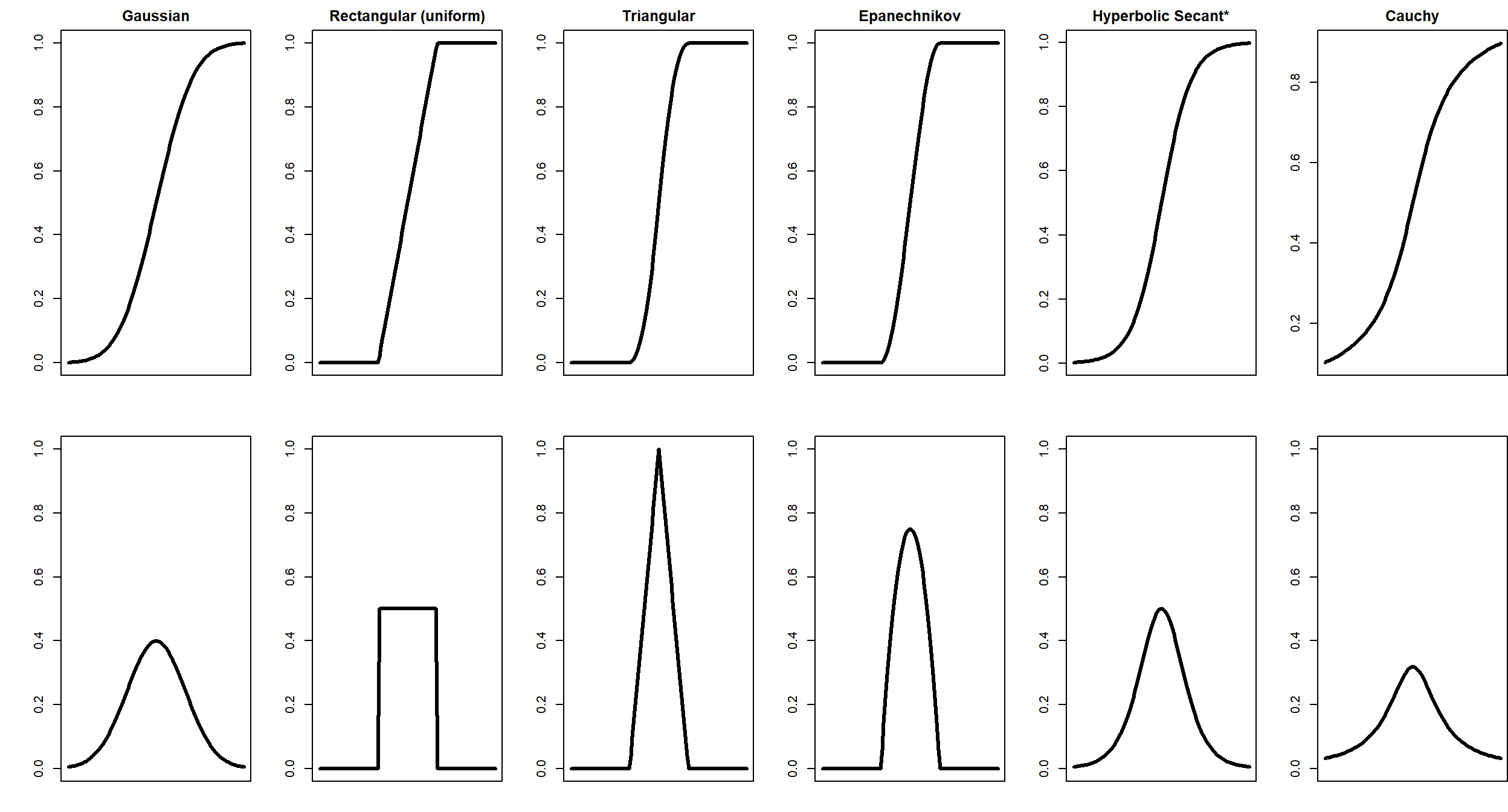
Recall that the kernel estimate of the CDF is \[ \hat{F}(x) = \frac{1}{n}\sum_{i=1}^n K(x,\text{bwt}_i,s) \] where \(K\) is a kernel function. In the previous module, you explored the Gaussian, rectagular (uniform), triangular, Epanechnikov, hypberbolic secant, and Cauchy kernels.
To find the estimated PDF from the kernel estimate of the CDF, let’s take the derivative. Let \(k\) be the derivate of \(K\) with respect to \(x\).
\[ \begin{aligned} \hat{f}(x) &= \frac{\hat{F}(x)}{dx}\\ &= \frac{1}{n}\sum_{i=1}^n \frac{dK(x,\text{bwt}_i,s)}{dx}\\ &= \frac{1}{n}\sum_{i=1}^n k(x,\text{bwt}_i,s)\\ \end{aligned} \]
The kernel functions in CDF form and PDF form are plotted below.
To generate the kernel estimate of the PDF of birth weight, we can write an R function similar to the function created for the CDF.
bwt <- MASS::birthwt$bwt
f <- function(x,s) rowMeans(outer(x,bwt,function(a,b) dnorm(a,b,s)))
hist(bwt, freq = FALSE, breaks = 25)
curve(f(x,250), add=TRUE, lwd = 3, col = "red")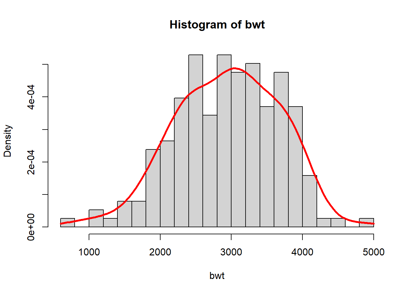
R also has ready-made commands for kernel density estimation.
f <- density(bwt, adjust = 1, kernel = "gaussian")
hist(bwt, freq = FALSE, breaks = 25)
lines(f, lwd = 3, col = "purple")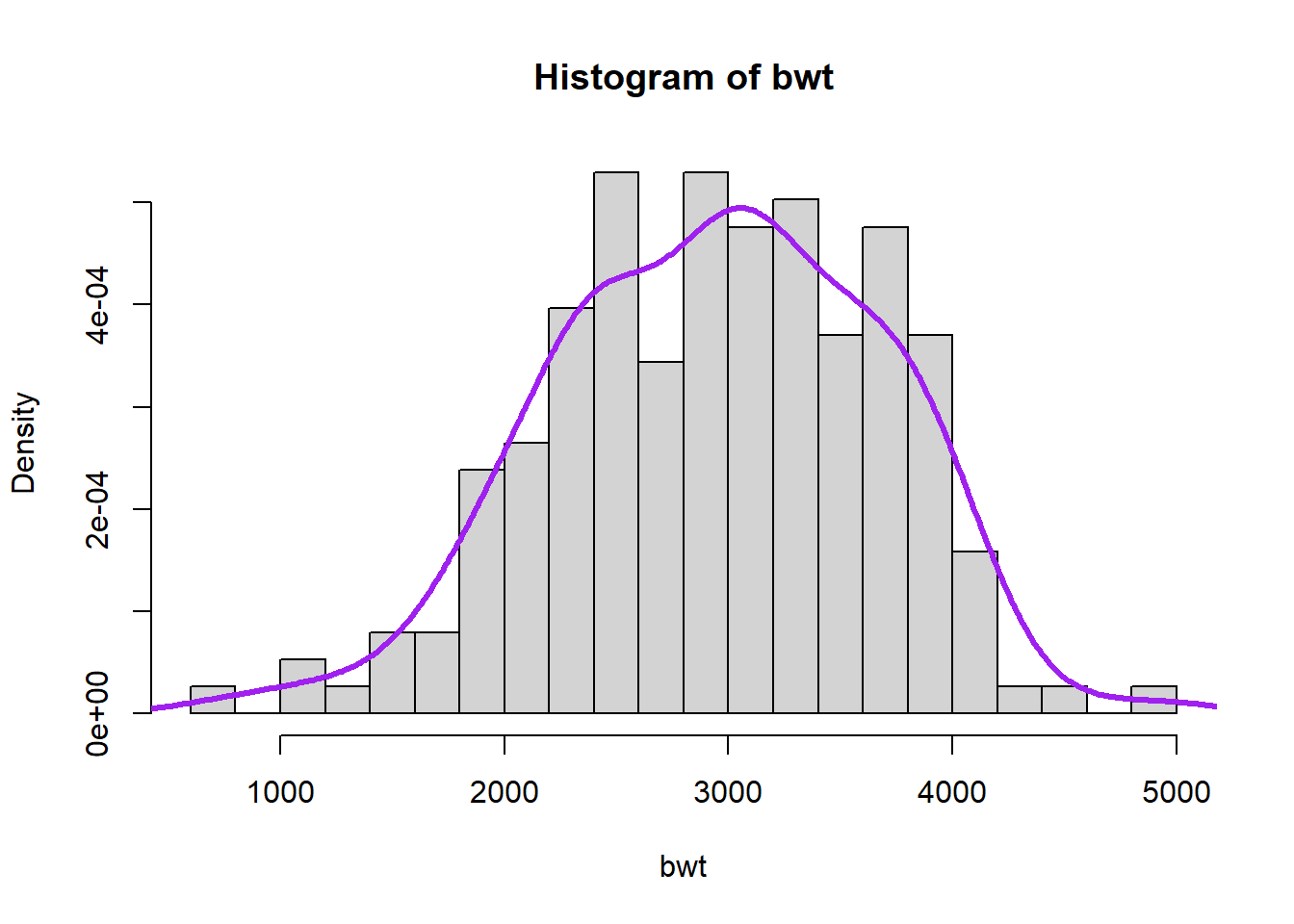
The density command incorporates methods for automatically selecting the smoothing parameter. The user can increase or decrease the degree of smoothing using the adjust input, with smaller values for less smoothing and larger values for more.
Interactive. Navigate here (link). Note: Typically CDFs and PDFs are on very different scales. The y-axis for a CDF goes from 0 to 1. The y-axis for a PDF can go from 0 to infinity. So that the CDF and PDF can be viewed on the same scale, the CDF has been multiplied by 0.001.
Hands on:
age variable) and overlay a density estimate using the Epanechnikov kernel.