
11 Method of moments
Recall that in this part of the text, we tackle the problem of constructing models (or updating beliefs) from data. Because data collection is also a source of uncertainty, we investigate how to appropariately propagate the uncertainty to the inferences (aka, answers to our questions) that we pulled from the models. Communicating the uncertainty associated with our answers will be key.
The goal of estimation is to find a probability model that describes the collected data so that, ultimately, we can answer questions about a larger population.
We noted that there are several ways to use the data to estimate a probability model.
Roadmap:
✓ Eyeball
✓ Kernel density estimation (nonparametric)
Today: Method of moments (parametric)
Next: Maximum likelihood (parametric)
Next: Bayesian posterior (parametric)
11.1 tl;dr; Method of moments
- Pick a parametric family.
- Match sample moments to model moments
11.1.1 Example: log creatinine
Consider the NHANES creatinine (mg/dL) data, on the log scale.
Hmisc::getHdata(nhgh)
scr <- nhgh$SCr
hist(log(scr), breaks=50, freq = FALSE)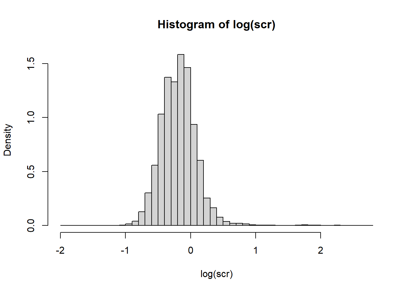
Suppose we model log creatinine with a normal distribution. There are two unknown parameters: \(\mu\) and \(\sigma\). Let’s pick the model parameter values so that the sample moments (sample mean and sample variance) match the model moments.
\[ \begin{align*} \text{sample mean} &\stackrel{set}{=} \text{model mean} \\ \text{sample variance} &\stackrel{set}{=} \text{model variance} \end{align*} \]
\[ \begin{align*} \bar{X} &\stackrel{set}{=} E[X] \\ S^2 &\stackrel{set}{=} V[X] \end{align*} \]
\[ \begin{align*} \frac{1}{n}\sum_{i=1}^n x_i &\stackrel{set}{=} \mu \\ \frac{1}{n-1}\sum_{i=1}^n (x_i-\bar{x})^2 &\stackrel{set}{=} \sigma^2 \end{align*} \]
mu_hat <- mean(log(scr), na.rm = TRUE)
sigma_hat <- sd(log(scr), na.rm = TRUE)
hist(log(scr), breaks=50, freq = FALSE)
curve(dnorm(x, mu_hat, sigma_hat), add = TRUE, lwd = 3, col = "red")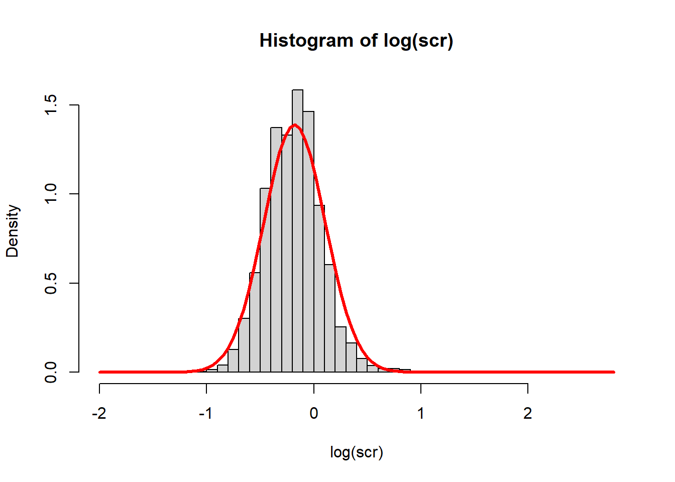
11.1.2 Example: creatinine
Consider the NHANES creatinine (mg/dL) data, modeled with a log normal distribution.
\[ \begin{align*} \text{sample mean} &\stackrel{set}{=} \text{model mean} \\ \text{sample variance} &\stackrel{set}{=} \text{model variance} \end{align*} \]
\[ \begin{align*} \bar{X} &\stackrel{set}{=} E[X] \\ S^2 &\stackrel{set}{=} V[X] \end{align*} \]
\[ \begin{align*} \frac{1}{n}\sum_{i=1}^n x_i &\stackrel{set}{=} e^{\mu + \sigma^2/2} \\ \frac{1}{n-1}\sum_{i=1}^n (x_i-\bar{x})^2 &\stackrel{set}{=} (e^{\sigma^2} - 1)e^{2\mu + \sigma^2} \end{align*} \]
The system of equations can be solved:
\[ \begin{align*} \hat{\sigma} &= \sqrt{\log \left( \frac{S^2}{\bar{X}^2} + 1\right)}\\ \hat{\mu} &= \log \frac{\bar{X}}{\sqrt{\frac{S^2}{\bar{X}^2} + 1}} \end{align*} \]
The method of moments solution can be compared to the historgram:
xbar <- mean(scr, na.rm = TRUE)
s2 <- var(scr, na.rm = TRUE)
mu_hat <- log(xbar/sqrt(s2/xbar^2 + 1))
sigma_hat <- sqrt(log(s2/xbar^2 + 1))
hist(scr[scr<5], breaks=50, freq = FALSE)
curve(dlnorm(x, mu_hat, sigma_hat), add = TRUE, lwd = 3, col = "blue")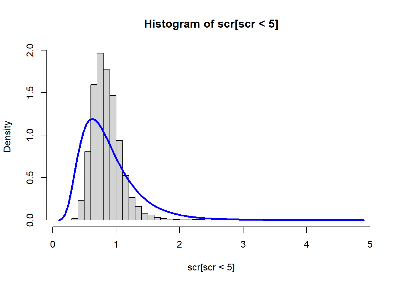
Sanity check. Do the model moments match the sample moments?
rlnorm(1000000,mu_hat, sigma_hat) |> mean(); xbar[1] 0.8789605[1] 0.8786266rlnorm(1000000,mu_hat, sigma_hat) |> var(); s2[1] 0.199126[1] 0.198236611.1.3 Example: creatinine with quantiles
Consider the NHANES creatinine (mg/dL) data, modeled with a log normal distribution using quantiles instead of moments.
\[ \begin{align*} \text{sample median} &\stackrel{set}{=} \text{model median} \\ \text{sample IQR} &\stackrel{set}{=} \text{model IQR} \end{align*} \]
\[ \begin{align*} \hat{Q_2} &\stackrel{set}{=} Q_2 \\ \hat{Q}_3 - \hat{Q}_1 &\stackrel{set}{=} Q_3 - Q_1 \end{align*} \]
\[ \begin{align*} \hat{Q_2} &\stackrel{set}{=} e^{\mu} \\ \hat{Q}_3 - \hat{Q}_1 &\stackrel{set}{=} e^{\mu + \sigma \Phi^{-1}(0.75)} - e^{\mu + \sigma \Phi^{-1}(0.25)} \end{align*} \]
qs <- quantile(scr, na.rm = TRUE)
mu_hat <- log(qs["50%"])
delta <- diff(qs[c("25%","75%")])
g <- function(s) delta*exp(-mu_hat) - (exp(s*qnorm(0.75)) - exp(s*qnorm(0.25)))
curve(g(x), .1, .3)
abline(h=0)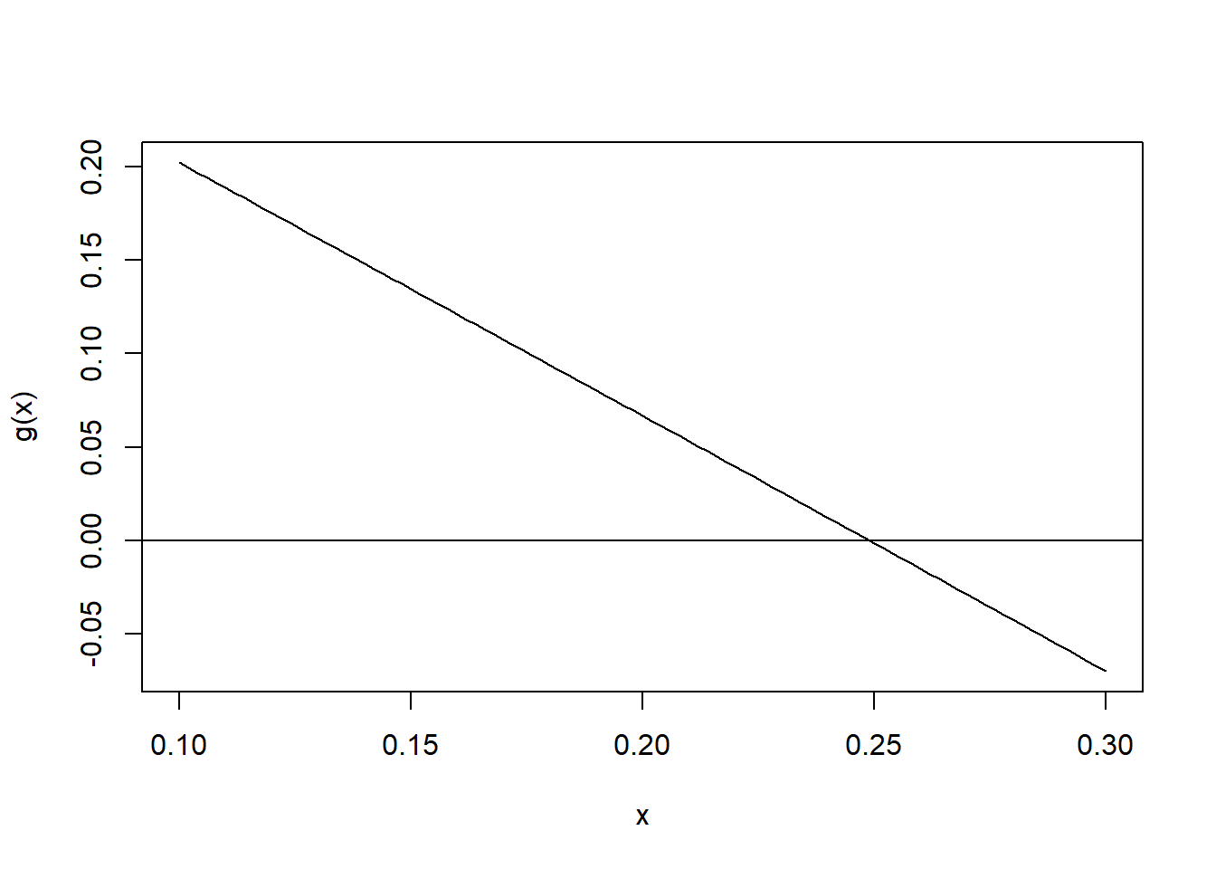
s_hat <- uniroot(g,c(.1,.3))$roothist(scr[scr<5], breaks=50, freq = FALSE)
curve(dlnorm(x, mu_hat, s_hat), add = TRUE, lwd = 3, col = "#03ac35")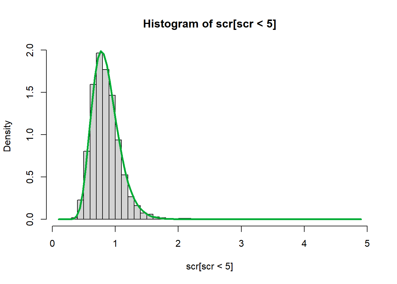
11.1.4 Example: Tricept skinfold
Take NHANES triceps skinfold measurement data.
hist(nhgh$tri, breaks = 50, freq = FALSE, main = "Tricept skinfold (mm)")
box()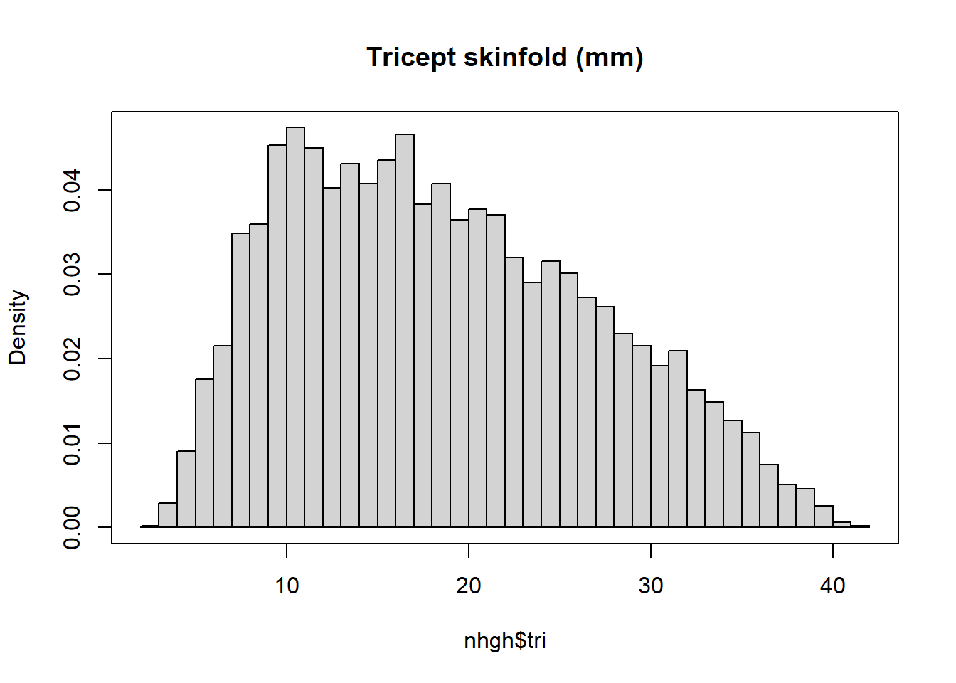
Suppose we model tricept skinfold measurements with a Weibull distribution. There are two unknown parameters to estimate: shape (\(\alpha\)) and scale (\(\sigma\)). Let’s pick the model parameter values so that the sample moments (sample mean and sample variance) match the model moments.
\[ \begin{align*} \text{sample mean} &\stackrel{set}{=} \text{model mean} \\ \text{sample variance} &\stackrel{set}{=} \text{model variance} \end{align*} \]
\[ \begin{align*} \bar{X} &\stackrel{set}{=} E[X] \\ S^2 &\stackrel{set}{=} V[X] \end{align*} \]
\[ \begin{align*} \frac{1}{n}\sum_{i=1}^n x_i &\stackrel{set}{=} \sigma\Gamma(1+1/\alpha) \\ \frac{1}{n-1}\sum_{i=1}^n (x_i-\bar{x})^2 &\stackrel{set}{=} \sigma^2\Gamma(1+2/\alpha) - \sigma^2\Gamma^2(1+1/\alpha) \end{align*} \]
There are two equations and two unknowns which can be solved by substitution/plotting/numerical methods.
\[ \begin{align*} \bar{X} &= \sigma\Gamma(1+1/\alpha) \\ S^2 &= \sigma^2\Gamma(1+2/\alpha) - \sigma^2\Gamma^2(1+1/\alpha) \end{align*} \]
A little manipulation leads to two expressions
\[ \begin{align*} \frac{\bar{X}^2}{S^2} &= \frac{\Gamma^2(1+1/\alpha)}{\Gamma(1+2/\alpha) + \Gamma^2(1+1/\alpha)} \quad (\sigma \text{ eliminated, can solve for } \alpha)\\ \hat{\sigma} &= \frac{\bar{X}}{\Gamma(1+1/\hat{\alpha})} \quad (\text{from first eqn above}) \end{align*} \]
xbar <- mean(nhgh$tri, na.rm = TRUE)
s2 <- var(nhgh$tri, na.rm = TRUE)
g <- function(a) 1/(gamma(1+2/a)/(gamma(1+1/a)^2) - 1) - xbar^2/s2
curve(g(x),1,4)
abline(h=0)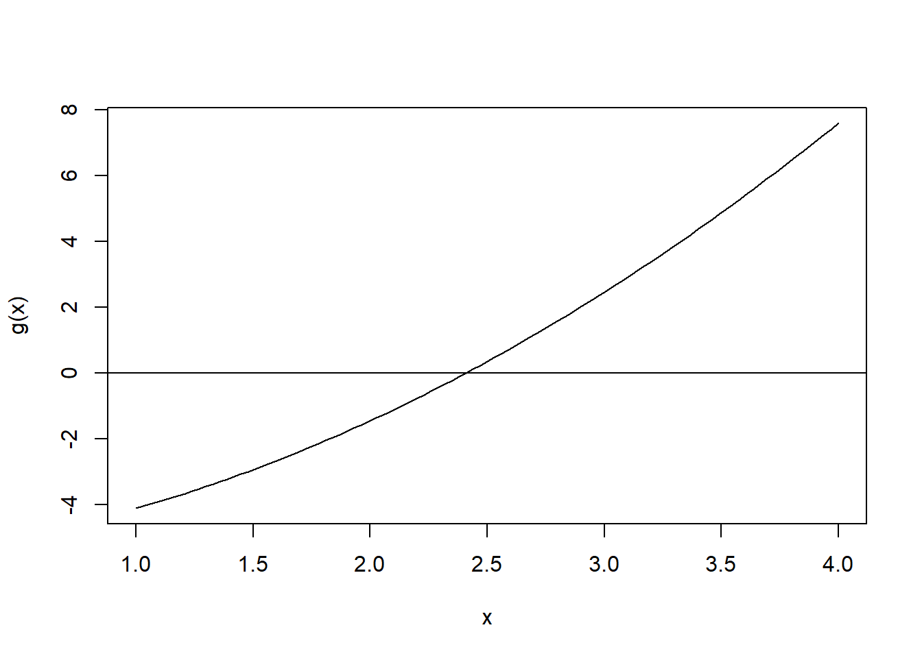
ahat <- uniroot(g,c(1,4))$root
sigmahat <- xbar/gamma(1+1/ahat)hist(nhgh$tri, breaks = 50, freq = FALSE, main = "Tricept skinfold (mm)", ylim = c(0,0.08))
box()
curve(dweibull(x, shape = ahat, scale = sigmahat), add = TRUE, col = "red", lwd = 3)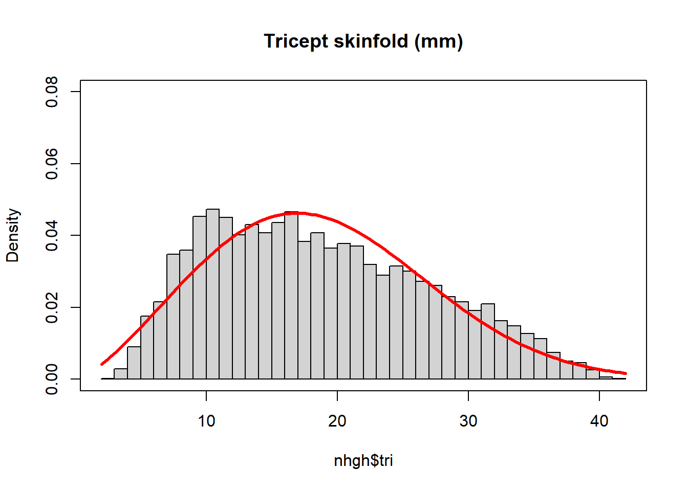
We can check to make sure the moments match up.
d1 <- rweibull(100000, shape = ahat, scale = sigmahat)
mean(d1); xbar
[1] 18.73137[1] 18.78773var(d1); s2[1] 69.19768[1] 69.212311.2 The bigger idea
The big idea of method of moments is to create a system of equations using moments. The bigger idea is to create a system of equations using any characteristic of the sample and model. For example, if moments do not exist, one might create a system of equations with quantiles like the median and interquartile range.
11.3 Steps for Method of Moments
Choose a parametric distribution, \(F_X(x|\theta)\). Identify the distribution parameters, \(\theta\)
Calculate/find distribution moments (need as many moments as distribution parameters), \(E[X^k]\) or \(E[(X - E[X])^k]\)
Calculate sample moments.
Create system of equations equating distribution moments to sample moments.
Solve system of equations for distribution parameters.
\(\hat{F}_X = F_X(x | \theta = \hat{\theta})\)
11.4 Example: BMI
bmi <- nhgh$bmi1a. Choose a parametric distribution, \(F_X(x|\theta)\) \[X \sim \text{gamma}(\text{shape}, \text{scale})\]
1b. Identify the distribution parameters, \(\theta\) \[\theta = (\text{shape},\ \text{scale})\]
2. Calculate/find distribution moments (need as many moments as distribution parameters), \(E[X^k]\) or \(E[(X - E[X])^k]\) \[E[X] = \text{shape}*\text{scale}\] \[V[X] = \text{shape}*\text{scale}^2\]
3. Calculate sample moments.
xbar <- mean(bmi) #28.32
s2 <- var(bmi)  #48.30
4. Create system of equations equating distribution moments to sample moments.
\[ \text{shape}*\text{scale} = \bar{X}\] \[ \text{shape}*\text{scale}^2 = s^2\]
5. Solve system of equations for distribution parameters. (In this example, we use the plug-in method.)
\[ \text{shape} = \frac{\bar{X}}{\text{scale}} \]
\[ \frac{\bar{X}}{\text{scale}}*\text{scale}^2 = s^2\]
\[ \text{scale} = \frac{s^2}{\bar{X}},\ \text{shape} = \frac{\bar{X}^2}{s^2}\]
shape_hat <- xbar^2/s2 #16.6
scale_hat <- s2/xbar  #1.7
\[ \hat{\theta} = (\widehat{\text{shape}}= 16.6,\ \widehat{\text{scale}} = 1.7)\]
6. \(\hat{F}_X = F_X(x | \theta = \hat{\theta})\)
Fbmi <- function(x){
pgamma(x, shape = shape_hat, scale = scale_hat)
}plot(ecdf(bmi))
curve(Fbmi(x), add = TRUE, col = "red", lwd = 3, main = "BMI")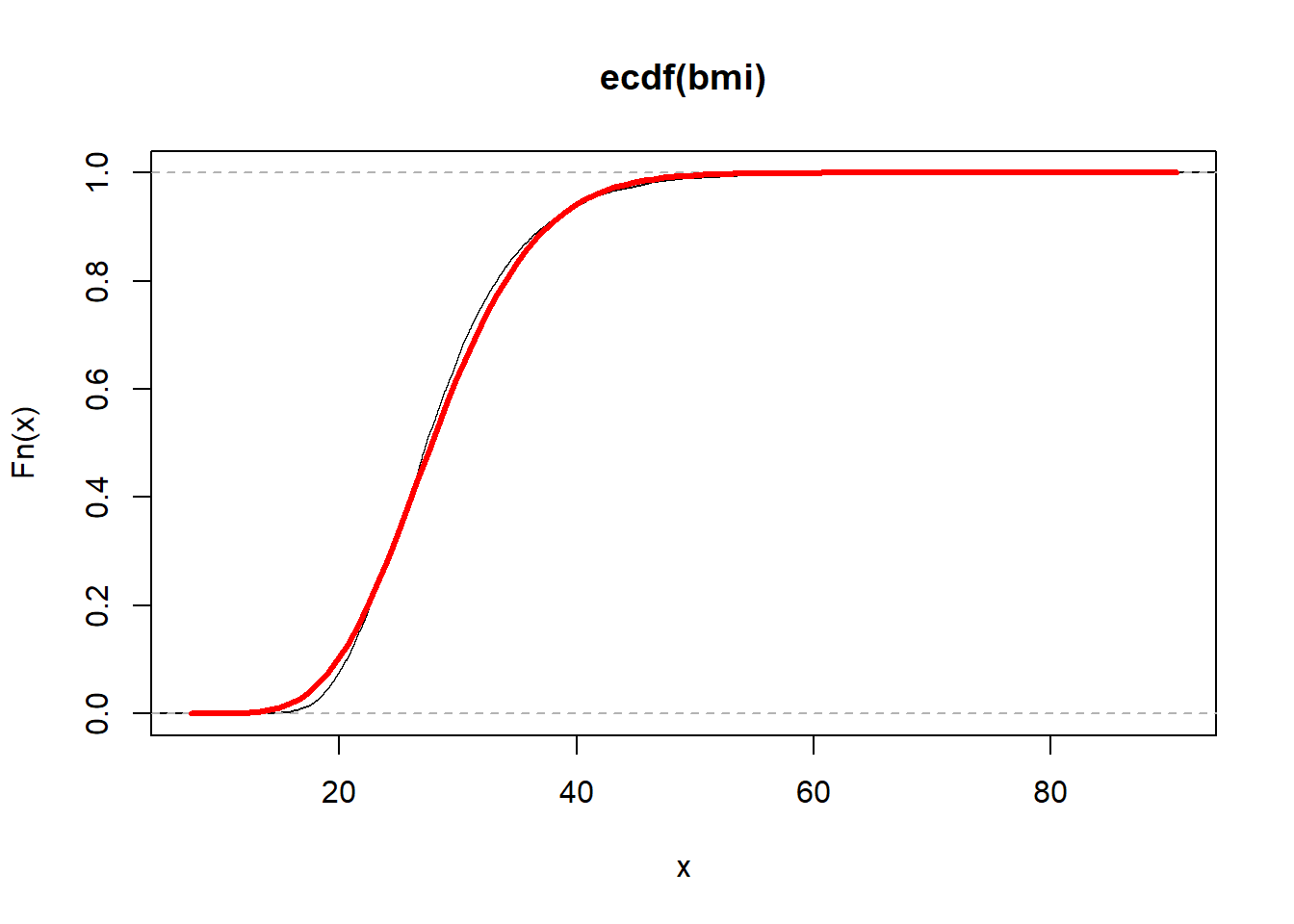
fbmi <- function(x){dgamma(x, shape = shape_hat, scale = scale_hat)}
hist(bmi, freq = FALSE, main = "BMI", breaks = 50)
curve(fbmi(x), add = TRUE, col = "blue", lwd = 3, main = "BMI")
11.5 Hands on
Estimate \(F_{\text{weight}}\) and \(f_{\text{weight}}\) from the NHANES dataset using the methods of moments. Generate plots of your estimates.