HW 8 - Discrete and continuous random variables

Question 1

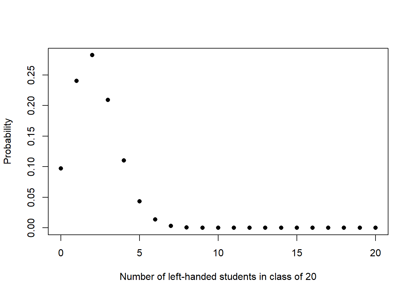
It is believed that about 11% of the population is left-handed. Generate a plot of the probability mass function for number of left-handed students in a class of 20.

Solution

x <- 0:20
p <- dbinom(x,20,0.11) # something else goes here
plot(x,p, xlab = "Number of left-handed students in class of 20", ylab = "Probability", pch = 16)

Question 2

Continuing from question 1, generate a plot of the cumulative probability function.

Solution

x <- 0:20
cp <- pbinom(x, 20, .11)
plot(x,cp, xlab = "Number of left-handed students in class of 20", ylab = "Cumulative probability", pch = 16)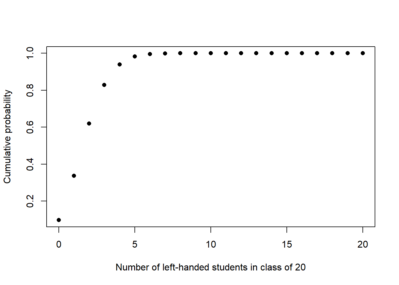

Question 3

Continuing from question 1, what is probability of 4 or more left-handed students in a class of size 20?

Solution

1 - pbinom(3, 20, .11)

[1] 0.170952

Question 4

Suppose a researcher is interested in enrolling 5 left-handed individuals into a study. Let \(M\) be the number of individuals the researcher must approach in order to contact 5 left-handed individuals.

Generate a plot of the pmf of \(M\).

Solution

\(M\) is a negative binomial random variable with stopping rule \(k=5\) and \(p=0.11\).

Note that \(M = R+k\) where \(R\) is the number of right handers contacted before the \(k^{th}\) left hander is contacted. Note that the dnbinom and pnbinom commands are parameterized for \(R = M-k\), which is why we input x-5 in the command below.

x <- 5:120
p <- dnbinom(x-5,5,0.11)
plot(x,p, xlab = "Number of encounters", ylab = "P(M=x)")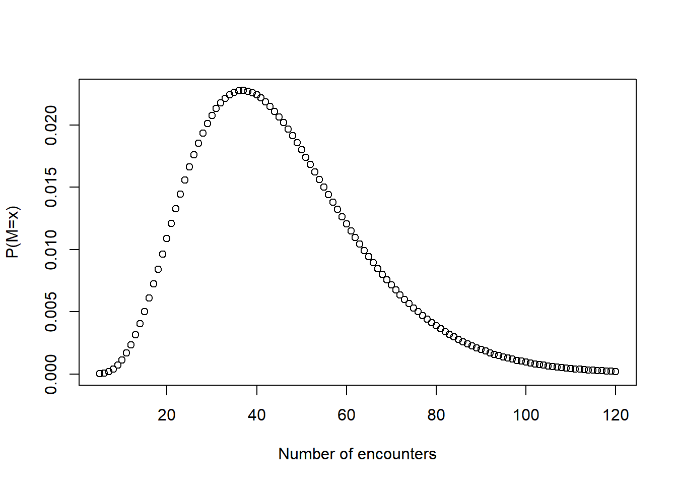

Question 5

Continuing question 4, generate a plot of the cdf of \(M\).

Solution

p <- pnbinom(x-5,5,0.11)
plot(x,p, xlab = "Number of encounters", ylab = "P(M <= x)")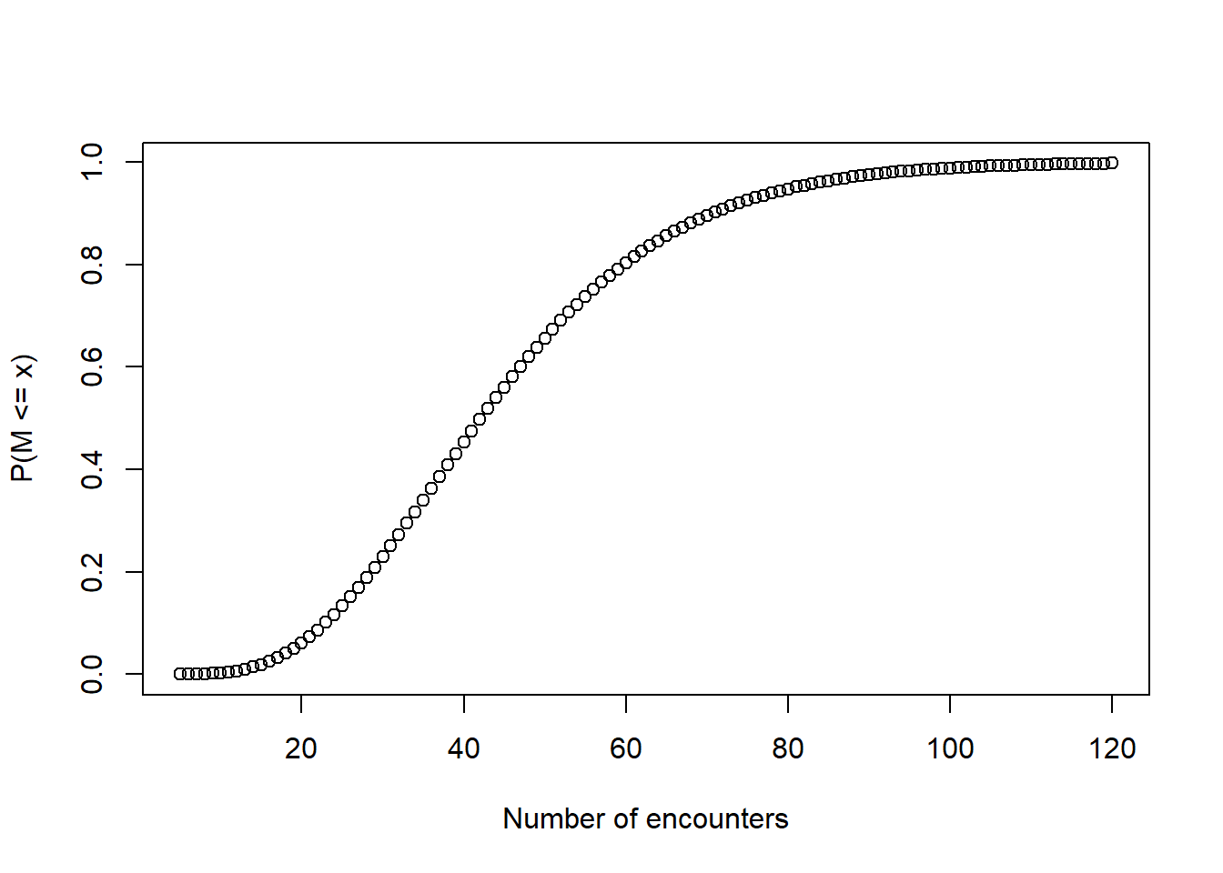

Question 6

Continuing question 4, the research only has funds to contact up to 60 individuals. What is the probability that the researcher will contact 5 left-handed individuals before funds are depleted?

Solution

pnbinom(60-5,5,.11)

[1] 0.803431

Question 7

Continuing question 4, on average, how many individuals will the researcher need to screen in order to contact 5 left-handed individuals?

Solution

The mathematical solution

\[ E[M] = E[R+5] = E[R] + 5 = \frac{k(1-p)}{p} + 5 = \frac{5(.89)}{.11} + 5 = 45.5 \]

The computational solution

set.seed(2309425)
m <- rnbinom(100000, 5, .11) + 5
mean(m)

[1] 45.49798

Question 8

Suppose infant birth weights are distributed normally with mean 3055 grams and standard deviation of 753 grams. If an infant is the \(98^{th}\) percentile for weight, what is the weight of the infant in grams?

Solution

The inverse of the CDF, the quantile function, maps cumulative left hand probabilities to quantiles.

# In grams
qnorm(0.98, 3055, 753)

[1] 4601.473

Question 9

The world health organization defines the threshold for low birth weight at 2500 grams. What proportion of infants are low birth weight, assuming the distribution from question 8?

Solution

\[ P(\text{birth weight} \leq 2500) = F(2500, \mu = 3055, \sigma = 753) = \text{\tt pnorm(2500, 3055, 753)} \]

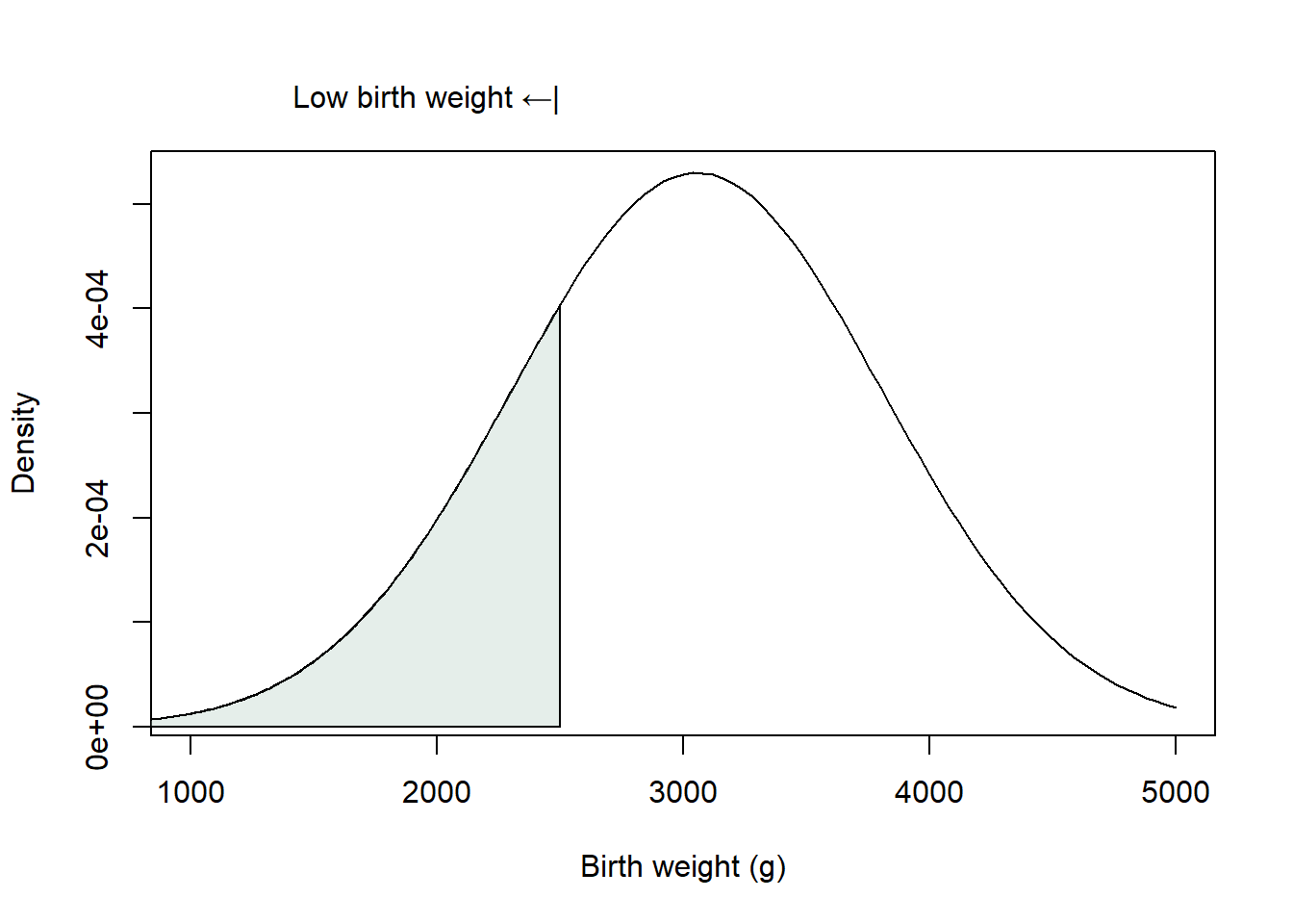
pnorm(2500, 3055, 753)

[1] 0.2305454

Question 10

Generate a plot of the birthweight density function, shading the region under the curve which corresponds to low birth weight infants.

Solution

curve(dnorm(x, 3055, 753), 1000, 5000, ylab = "Density", xlab = "Birth weight (g)")
x <- seq(0, 2500, length=200)
y <- dnorm(x, 3055, 753)
polygon(c(0,x,2500), c(0,y,0), col = "#abcabc50")
axis(3,2500,"Low birth weight ←|",hadj = 1,tick=FALSE)