Problem 1: Exponential Distribution - Estimating the Rate Parameter
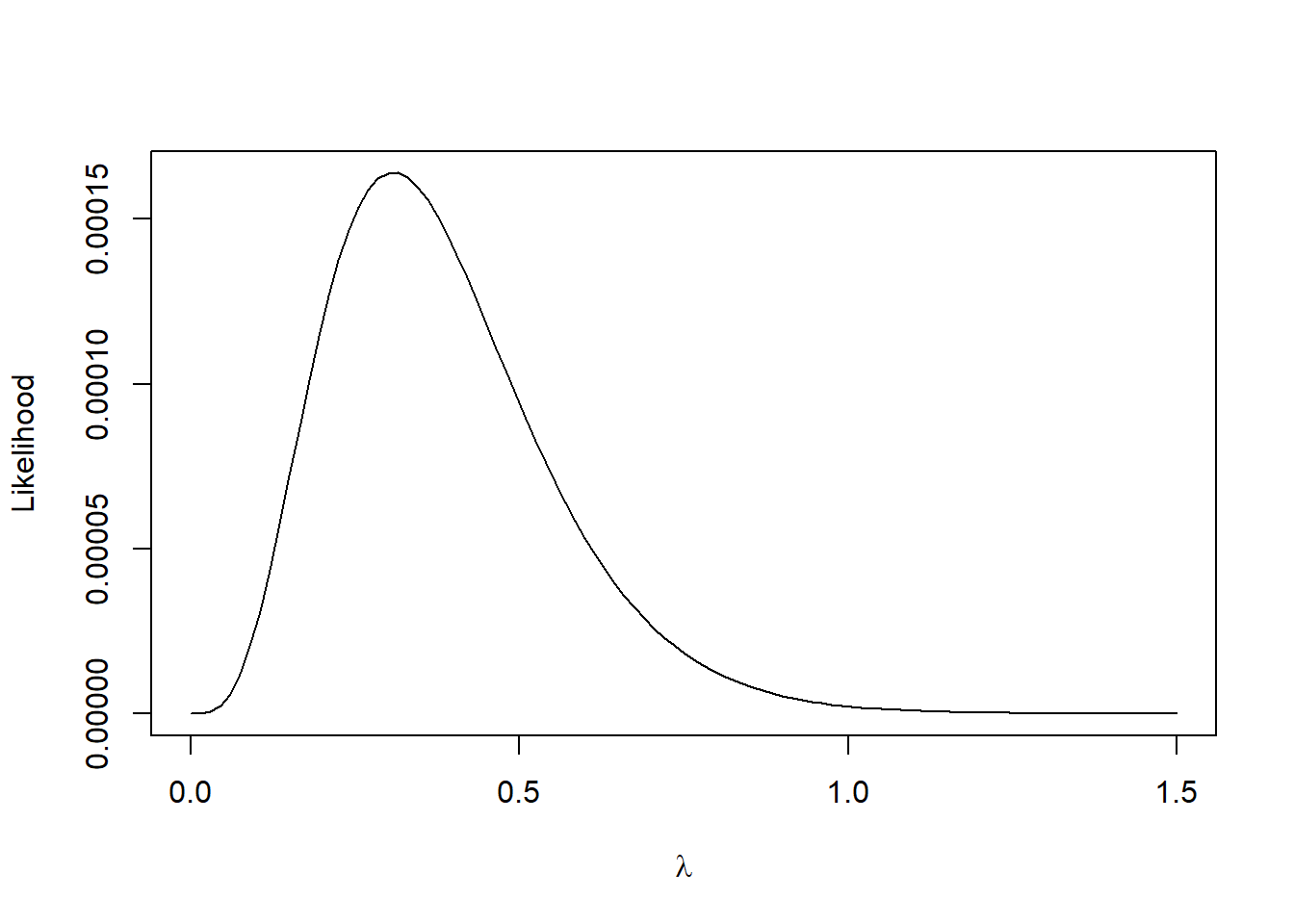
You observe the following waiting times (in minutes) for a bus: 2.5, 5.1, 1.8, 3.6. Assuming the waiting times follow an exponential distribution, estimate the rate parameter (\(\lambda\)) using MLE.
Solution
To construct the likelihood, we need the PDF of the exponential distribution. It is
\[
f(x) = \lambda \exp (-\lambda x)
\]
In R, this is the dexp function.
The likelihood is the product of the PDFs evaluated at the observed waiting times.
# MLE specific optimizersuppressPackageStartupMessages(require(stats4))o2 <-mle(function(x){negloglik(x,data = data)}, list(x =1))
Warning in FUN(X, Y, ...): NaNs produced
Warning in FUN(X, Y, ...): NaNs produced
Warning in FUN(X, Y, ...): NaNs produced
Warning in FUN(X, Y, ...): NaNs produced
Warning in FUN(X, Y, ...): NaNs produced
summary(o2)
Maximum likelihood estimation
Call:
mle(minuslogl = function(x) {
negloglik(x, data = data)
}, start = list(x = 1))
Coefficients:
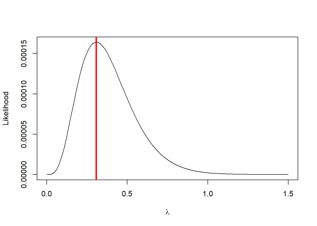
Estimate Std. Error
x 0.3076925 0.1538446
-2 log L: 17.42924
Problem 2: Normal Distribution - Estimating Mean and Variance
A sample of student heights (in inches) is: 65, 68, 72, 63, 70. Estimate the mean (\(\mu\)) and variance (\(\sigma^2\)) of the height distribution using MLE, assuming heights are normally distributed.
Solution
Like problem 1, this can be solved with calculus or numerically. The course notes already show both, so we skip those details.
data <-c(65, 68, 72, 63, 70)n <-length(data)mu_hat <-mean(data)sigma2_hat <-var(data) # Technically, the MLE estimate is var(data)*(n-1)/n. Note (n-1)/n goes to 1 as n gets large, so it is often ignoredc(mu_hat = mu_hat, sigma2_hat = sigma2_hat, sigma2_hat_corrected = sigma2_hat*(n-1)/n)
# Another command for normal# Note that lm give the uncorrected estimate for sigma (without the square)lm1 <-lm(data ~1)summary(lm1)
Call:
lm(formula = data ~ 1)

Residuals:
   1    2    3    4    5
-2.6  0.4  4.4 -4.6  2.4

Coefficients:
            Estimate Std. Error t value Pr(>|t|)
(Intercept)   67.600      1.631   41.45 2.03e-06 ***
---
Signif. codes:  0 '***' 0.001 '**' 0.01 '*' 0.05 '.' 0.1 ' ' 1

Residual standard error: 3.647 on 4 degrees of freedom
Problem 3: Poisson Distribution - Estimating the Average Number of Events
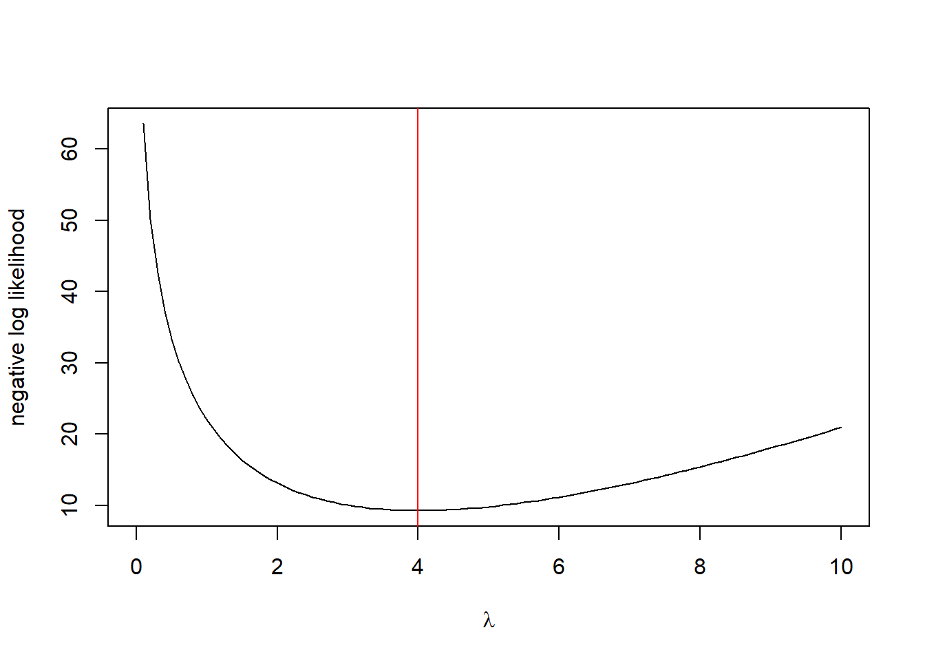
You count the number of cars passing a certain point on a road per minute for 5 minutes and get: 3, 5, 2, 4, 6. Estimate the average number of cars passing per minute (\(\lambda\)) using MLE, assuming a Poisson distribution.
Solution
Using Calculus: We construct the likelihood function (\(L(\lambda)\)), form the log likelihood function (\(\ell(\lambda)\)), calculate the derivative (\(\ell'(\lambda)\)), and finally find the root of the derivative.
# General purpose optimizeroptim(1,logliklihood, data = data, method ="Brent", lower =0, upper =100)
$par
[1] 4

$value
[1] 9.303816

$counts
function gradient
      NA       NA

$convergence
[1] 0

$message
NULL
# Poisson regression command gives log(lambda), which is why we exp the resultg1 <-glm(data ~1, family = poisson)summary(g1)
Call:
glm(formula = data ~ 1, family = poisson)

Coefficients:
            Estimate Std. Error z value Pr(>|z|)
(Intercept)   1.3863     0.2236     6.2 5.66e-10 ***
---
Signif. codes:  0 '***' 0.001 '**' 0.01 '*' 0.05 '.' 0.1 ' ' 1

(Dispersion parameter for poisson family taken to be 1)

    Null deviance: 2.5983  on 4  degrees of freedom
Residual deviance: 2.5983  on 4  degrees of freedom
AIC: 20.608

Number of Fisher Scoring iterations: 4
exp(coef(g1))
(Intercept)
          4
Problem 4: Uniform Distribution - Estimating the Upper Bound
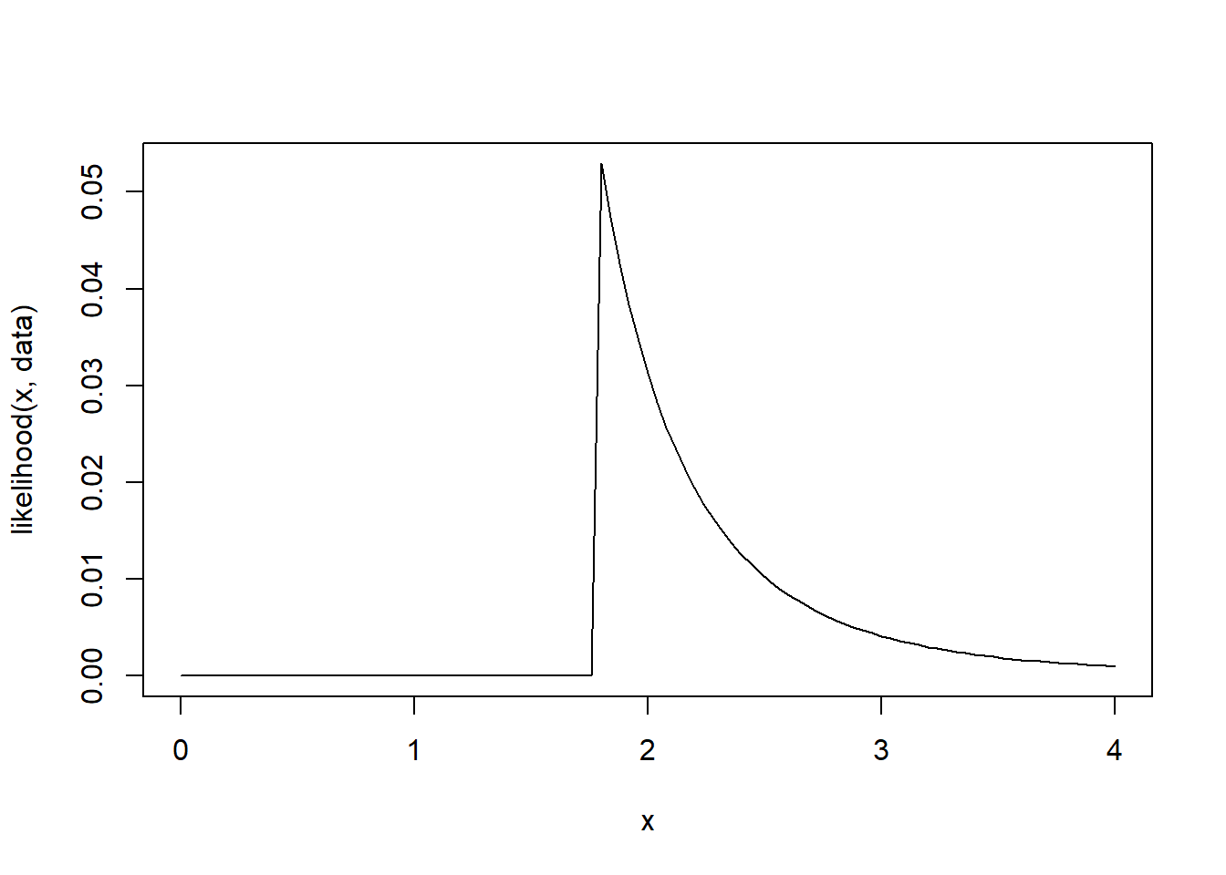
You have the following measurements of the length (in cm) of a manufactured part: 1.2, 1.8, 1.5, 1.7, 1.3. Assuming the lengths are uniformly distributed between 0 and \(\theta\), find the MLE for \(\theta\).
Solution
Calculus:
The PDF is \[
f(x) = \left\{ \begin{array}{ll} \frac{1}{\theta} & 0 < x \leq \theta \\ 0 & \text{otherwise} \end{array} \right.
\]
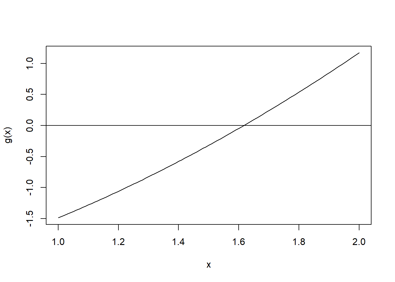
data <-c(1.2, 1.8, 1.5, 1.7, 1.3)likelihood <-function(theta, data){ ub <-max(data) n <-length(data) out <-1/theta^n out[theta < ub] <-0 out}curve(likelihood(x, data),0,4)
Notice that the likelihood is not differentiable at the maximum. Also note that the function is only non-zero for values of \(\theta\) greater than the maximum observed value. The maximum likelihood solution is
yy <- yyy[y<=0] <-0.0001# Weibull must have y strictly greater than 0negloglike<-function(a,sigma){-sum(dweibull(yy,shape = a, scale = sigma, log =TRUE))}m1 <-mle(negloglike, lower =c(0,0), start =c(1,1))m1
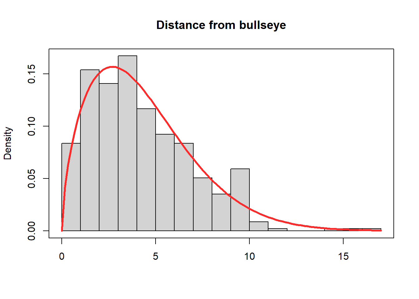
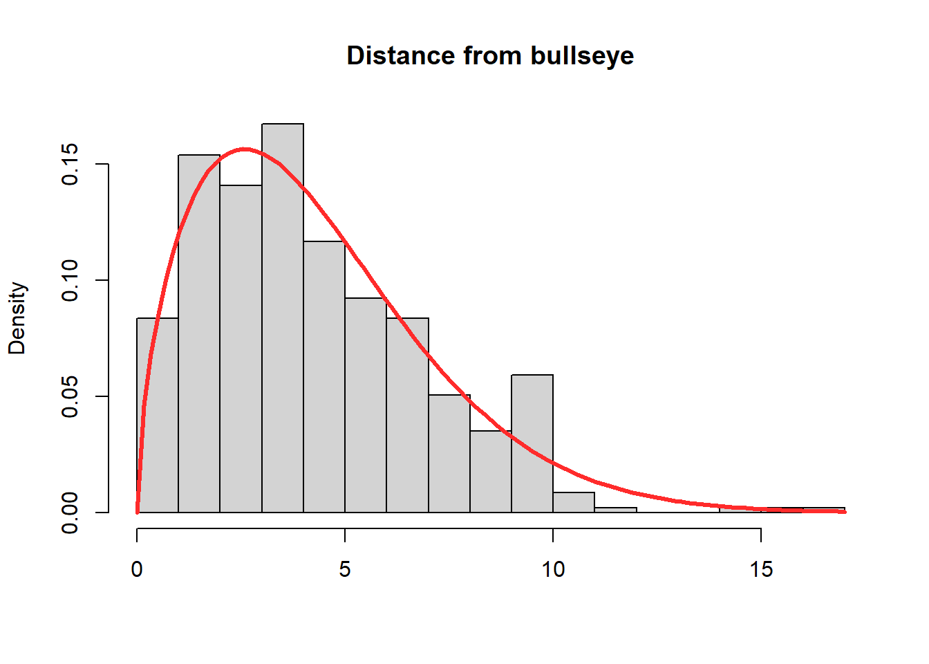
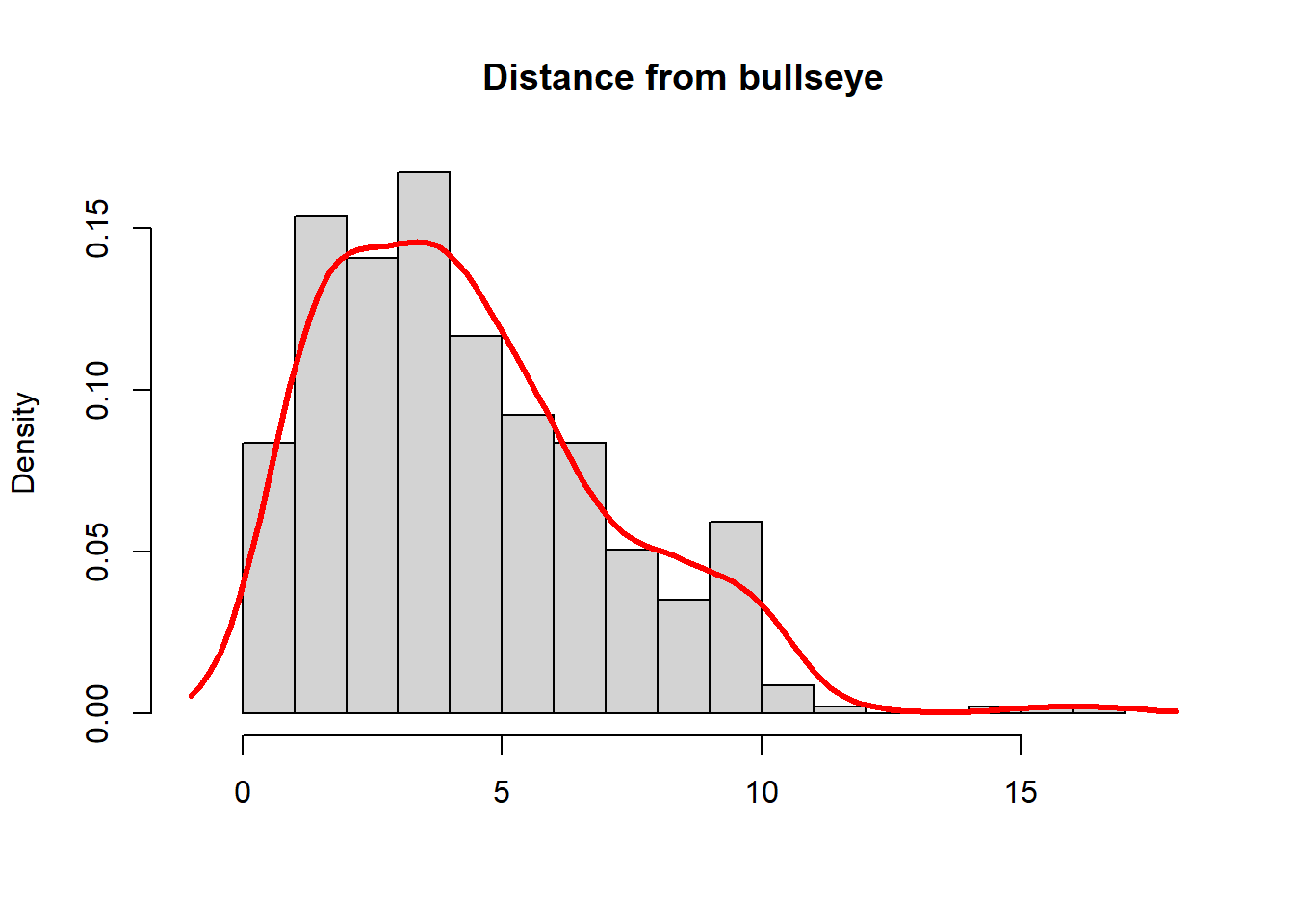
# Built in commandsd1 <-density(y, kernel ="g", bw ="SJ", adjust =1.4)hist(y, breaks=20,freq =FALSE, main ="Distance from bullseye", xlab="", xlim =range(y) +c(-1,+1))lines(d1, lwd =3, col ="#ff2b2b")box()
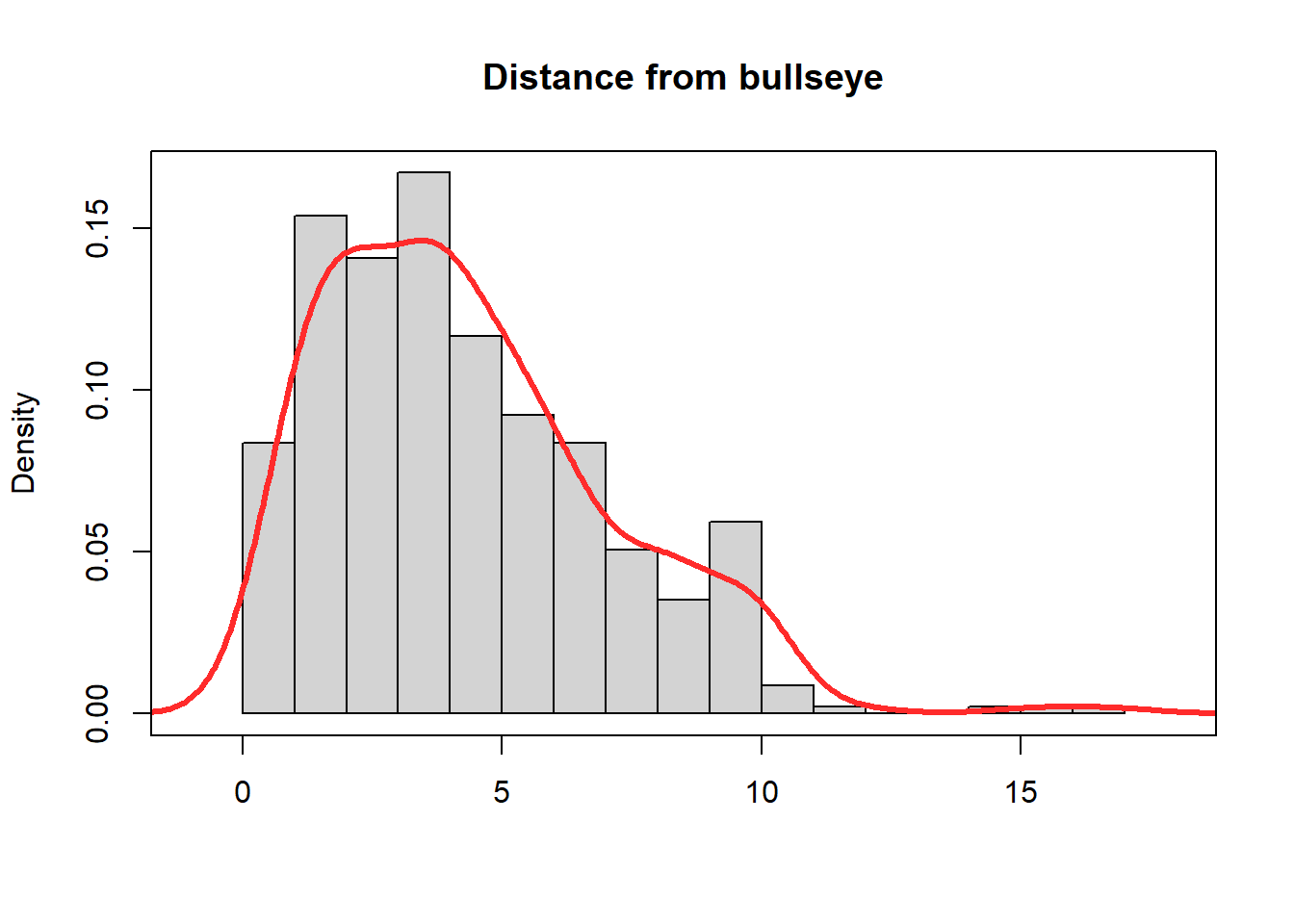
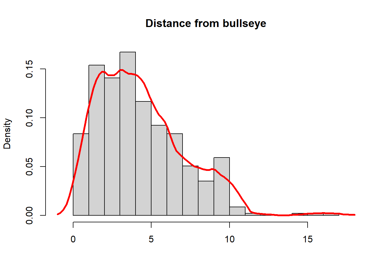
# Built in commandsd1 <-density(y, kernel ="e")hist(y, breaks=20,freq =FALSE, main ="Distance from bullseye", xlab="", xlim =range(y) +c(-1,+1))lines(d1, lwd =3, col ="#ff2b2b")box()