The National Health and Nutrition Examination Survey has been conducted since 1971 by the National Center for Health Statistics. The survey collects demographic, socioeconomic, dietary, and health data. The nhgh data available from the Hmisc package is a sample of responses from the survey. The data dictionary is here (link). We use this data to show how one might generate summary tables and visualizations in R.
Hmisc::getHdata(nhgh)# Peek at the datanhgh |>head()
    seqn    sex      age                 re        income tx dx    wt    ht
1  51624   male 34.16667 Non-Hispanic White [25000,35000)  0  0  87.4 164.7
3  51626   male 16.83333 Non-Hispanic Black [45000,55000)  0  0  72.3 181.3
5  51628 female 60.16667 Non-Hispanic Black [10000,15000)  1  1 116.8 166.0
6  51629   male 26.08333   Mexican American [25000,35000)  0  0  97.6 173.0
7  51630 female 49.66667 Non-Hispanic White [35000,45000)  0  0  86.7 168.4
10 51633   male 80.00000 Non-Hispanic White [15000,20000)  0  1  79.1 174.3
     bmi  leg arml armc waist  tri  sub  gh albumin bun  SCr
1  32.22 41.5 40.0 36.4 100.4 16.4 24.9 5.2     4.8   6 0.94
3  22.00 42.0 39.5 26.6  74.7 10.2 10.5 5.7     4.6   9 0.89
5  42.39 35.3 39.0 42.2 118.2 29.6 35.6 6.0     3.9  10 1.11
6  32.61 41.7 38.7 37.0 103.7 19.0 23.2 5.1     4.2   8 0.80
7  30.57 37.5 36.1 33.3 107.8 30.3 28.0 5.3     4.3  13 0.79
10 26.04 42.8 40.0 30.2  91.1  8.6 15.2 5.4     4.3  16 0.83
5.2 Summary tables
There are many, many table making packages in R. Here are a few options.
There are a few binary variables in the dataset, including sex, tx (using insulin or diabetes medications), and dx (diagnosed with diabetes or pre-diabetes). A simple tabular summary of the data is the counts and proportions.
We can add dx and tx directly to the table. Note the following:
The variable labels for dx and tx were automatically added to the table.
The command did not calculate the count and percentage for each group. Rather, it gave the output that is generated for a continuous varable.
table1(~ sex + dx + tx, data=nhgh)
Overall (N=6795)
sex
male
3372 (49.6%)
female
3423 (50.4%)
Diagnosed with DM or Pre-DM
Mean (SD)
0.135 (0.341)
Median [Min, Max]
0 [0, 1.00]
On Insulin or Diabetes Meds
Mean (SD)
0.0918 (0.289)
Median [Min, Max]
0 [0, 1.00]
Where did the labels come from? Why did the command generate the output for a continuous variable?
The label of the variable is stored as meta data. If we peek at the structure of the dataframe, we see the following info:
str(nhgh[,c("dx","tx")])
'data.frame':   6795 obs. of  2 variables:
 $ dx: 'labelled' int  0 0 1 0 0 1 1 0 0 1 ...
  ..- attr(*, "label")= chr "Diagnosed with DM or Pre-DM"
 $ tx: 'labelled' int  0 0 1 0 0 0 1 0 0 1 ...
  ..- attr(*, "label")= chr "On Insulin or Diabetes Meds"
Notice that the label attribute is specified for both variables. This is the metadata that the table1 command is using when it creates the table. Suppose we wanted to tweak the label.
label(nhgh$tx) <-"Using insulin or diabetes medications"table1(~ sex + dx + tx, data=nhgh)
Overall (N=6795)
sex
male
3372 (49.6%)
female
3423 (50.4%)
Diagnosed with DM or Pre-DM
Mean (SD)
0.135 (0.341)
Median [Min, Max]
0 [0, 1.00]
Using insulin or diabetes medications
Mean (SD)
0.0918 (0.289)
Median [Min, Max]
0 [0, 1.00]
Also note that tx and dx are listed as int variables. For table1 to treat tx and dx as categorical, binary variables, we need to change the variable type from integer to factor. Here, we keep the original data in-tack and add tx_f and dx_f.
Often, we need to stratify a summary table. For example, suppose we wanted to compare those diagnosed with diabetes vs those not diagnosed. We can use the | syntax in the table formula.
table1(~ sex + tx_f + age + wt | dx_f, data=nhgh)
No (N=5881)
Yes (N=914)
Overall (N=6795)
sex
male
2927 (49.8%)
445 (48.7%)
3372 (49.6%)
female
2954 (50.2%)
469 (51.3%)
3423 (50.4%)
Using insulin or diabetes medications
No
5864 (99.7%)
307 (33.6%)
6171 (90.8%)
Yes
17 (0.3%)
607 (66.4%)
624 (9.2%)
Age (years)
Mean (SD)
41.8 (20.3)
60.0 (15.1)
44.3 (20.6)
Median [Min, Max]
40.3 [12.0, 80.0]
62.1 [12.6, 80.0]
43.8 [12.0, 80.0]
Weight (kg)
Mean (SD)
77.7 (21.1)
89.8 (24.4)
79.4 (21.9)
Median [Min, Max]
74.9 [28.0, 239]
86.6 [37.0, 231]
76.3 [28.0, 239]
Notice that the labels may need to be different or a header added to the table. The reader will not know what Yes and No refer to.
table1(~ sex + tx_f + age + wt | dx_f, data=nhgh, caption =label(nhgh$dx_f))
Diagnosed with DM or Pre-DM
No (N=5881)
Yes (N=914)
Overall (N=6795)
sex
male
2927 (49.8%)
445 (48.7%)
3372 (49.6%)
female
2954 (50.2%)
469 (51.3%)
3423 (50.4%)
Using insulin or diabetes medications
No
5864 (99.7%)
307 (33.6%)
6171 (90.8%)
Yes
17 (0.3%)
607 (66.4%)
624 (9.2%)
Age (years)
Mean (SD)
41.8 (20.3)
60.0 (15.1)
44.3 (20.6)
Median [Min, Max]
40.3 [12.0, 80.0]
62.1 [12.6, 80.0]
43.8 [12.0, 80.0]
Weight (kg)
Mean (SD)
77.7 (21.1)
89.8 (24.4)
79.4 (21.9)
Median [Min, Max]
74.9 [28.0, 239]
86.6 [37.0, 231]
76.3 [28.0, 239]
5.3 Summary visualizations
When creating visualizations, the first step is to answer the following question:
What do I want my reader to glean from the visualization?
The answer to this question will dictate what and how you create the visualization. If the goal is a general summary, a simple expression of the raw data distribution is perfectly adequate. If the goal is comparison between groups, the summary measures to compare should be side-by-side.
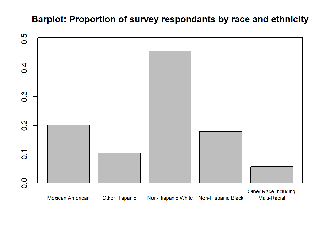
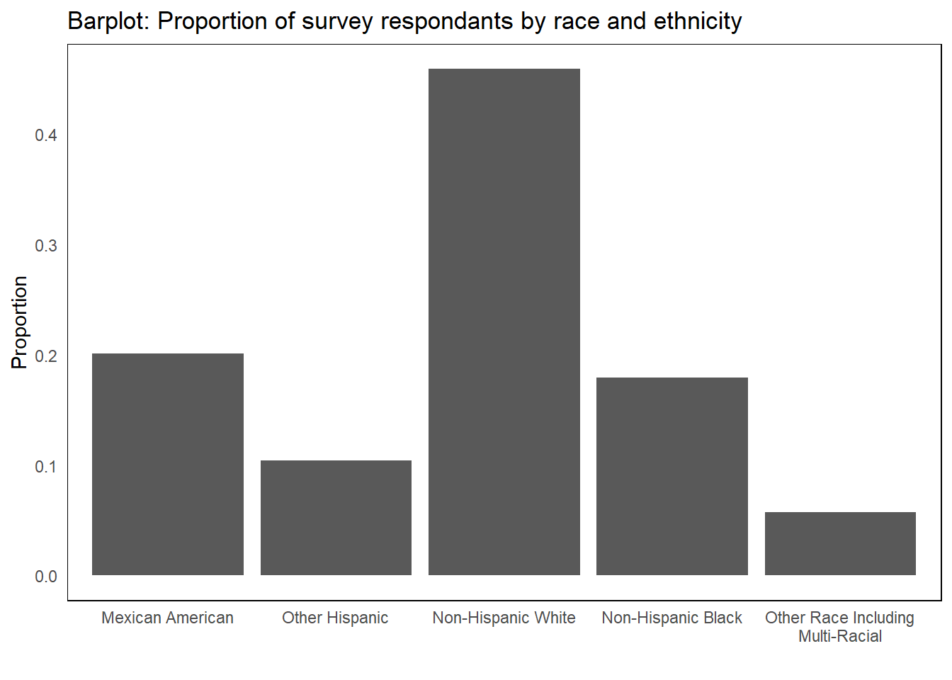
suppressPackageStartupMessages(library(ggplot2))t2 <-as.data.frame(t1)names(t2) <-c("re", "p")# Create the bar plotggplot(t2, aes(x = re, y = p)) +geom_bar(stat ="identity") +labs(title ="Barplot: Proportion of survey respondants by race and ethnicity", x ="", y ="Proportion") +theme_minimal() +theme(panel.border =element_rect(colour ="black", fill =NA),panel.grid =element_blank())
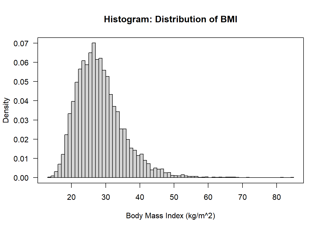
get_label <-function(x){ uu <-ifelse(has.units(x), gsub("U",units(x),"(U)"), "") ll <-ifelse(has.label(x), label(x), "No label")paste(ll,uu)}hist( nhgh$bmi , breaks =100 , freq =FALSE , main ="Histogram: Distribution of BMI" , xlab =get_label(nhgh$bmi) , las =1)box()
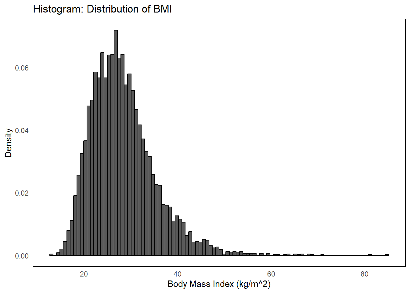
ggplot(nhgh, aes(x = bmi)) +geom_histogram(aes(y =after_stat(density)), bins =100, color ="black") +labs(title ="Histogram: Distribution of BMI", x =get_label(nhgh$bmi), y ="Density") +theme_minimal() +theme(panel.border =element_rect(colour ="black", fill =NA),panel.grid =element_blank() )
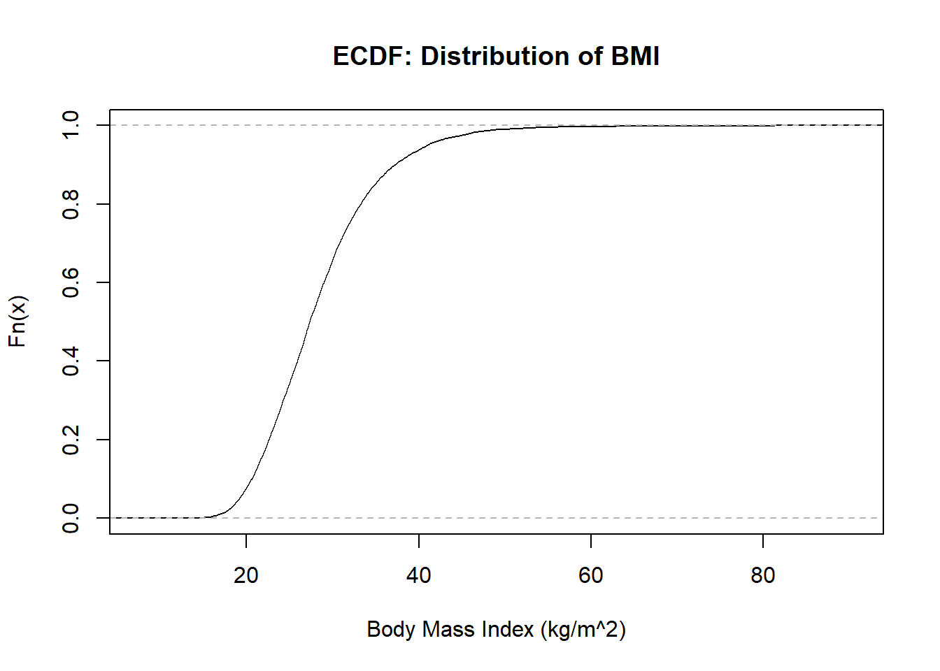
plot(ecdf(nhgh$bmi), main ="ECDF: Distribution of BMI", xlab =get_label(nhgh$bmi))box()
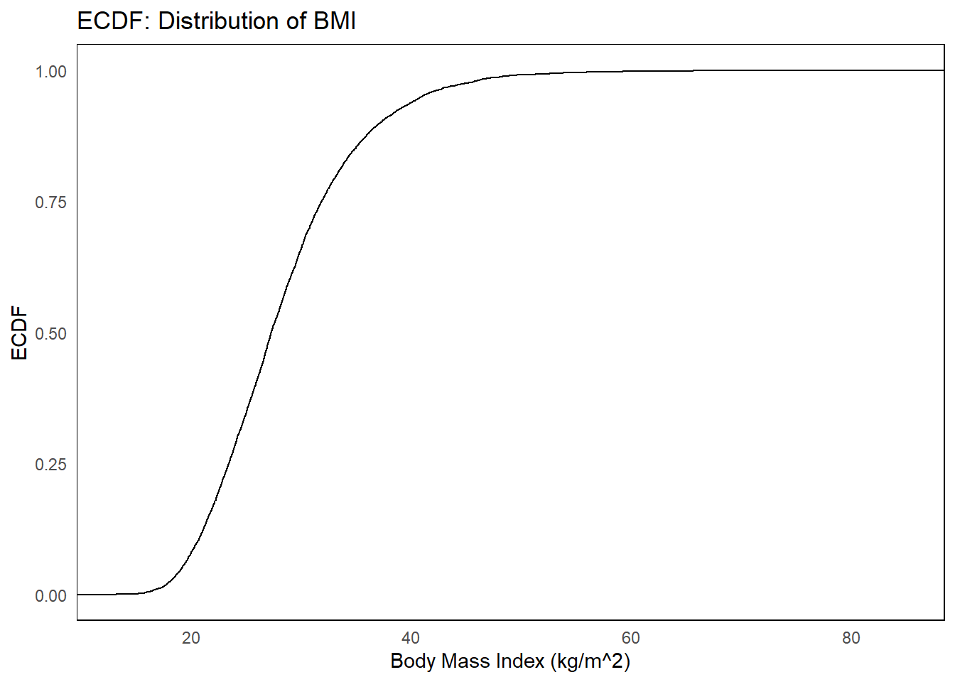
ggplot(nhgh, aes(x = bmi)) +stat_ecdf(geom ="step") +labs(title ="ECDF: Distribution of BMI", x =get_label(nhgh$bmi), y ="ECDF") +theme_minimal() +theme(panel.border =element_rect(colour ="black", fill =NA),panel.grid =element_blank() )
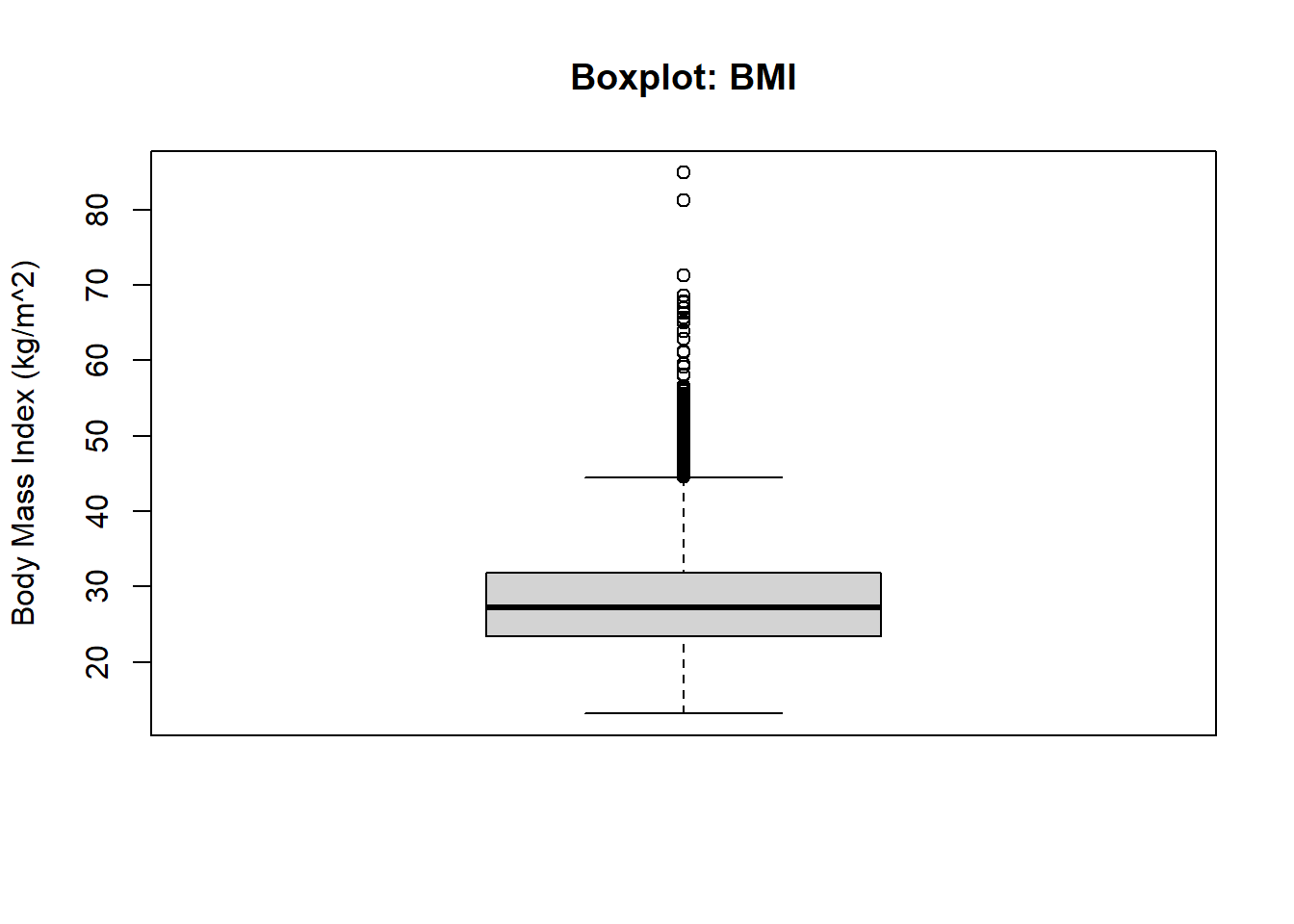
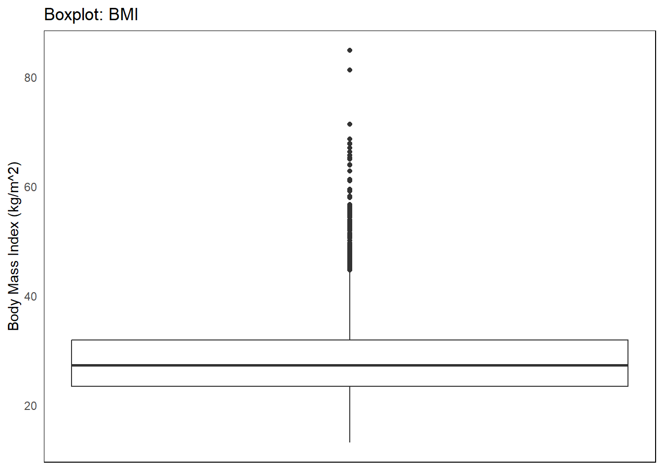
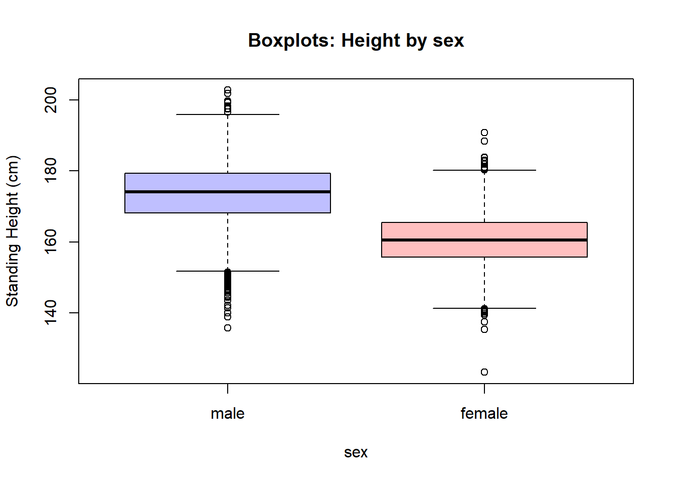
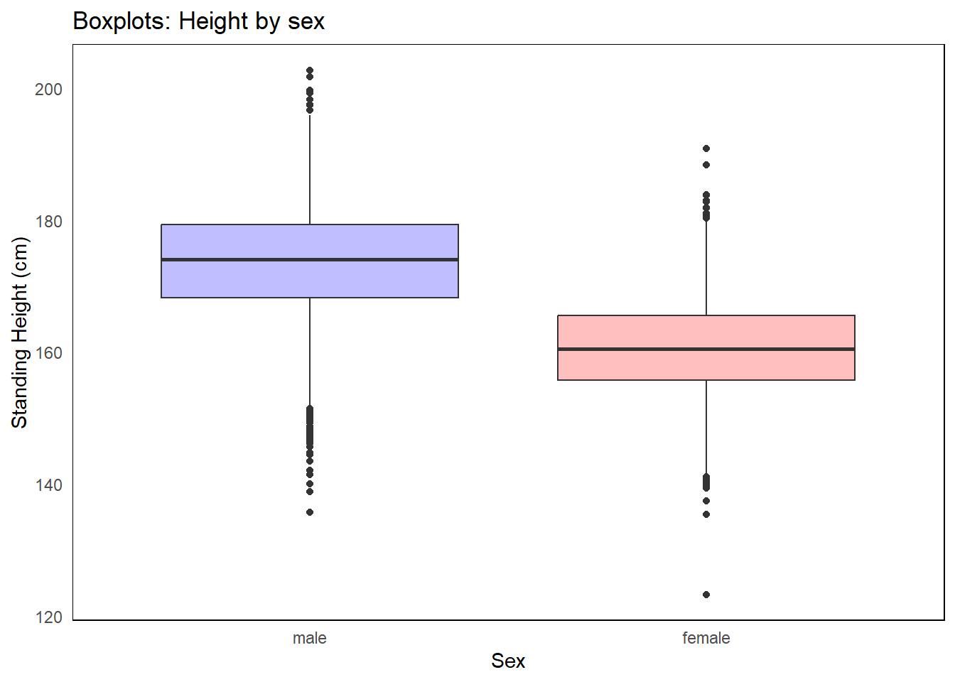
The box plot is a 5 number summary of the distribution. It is most often used when comparing distributions across groups.
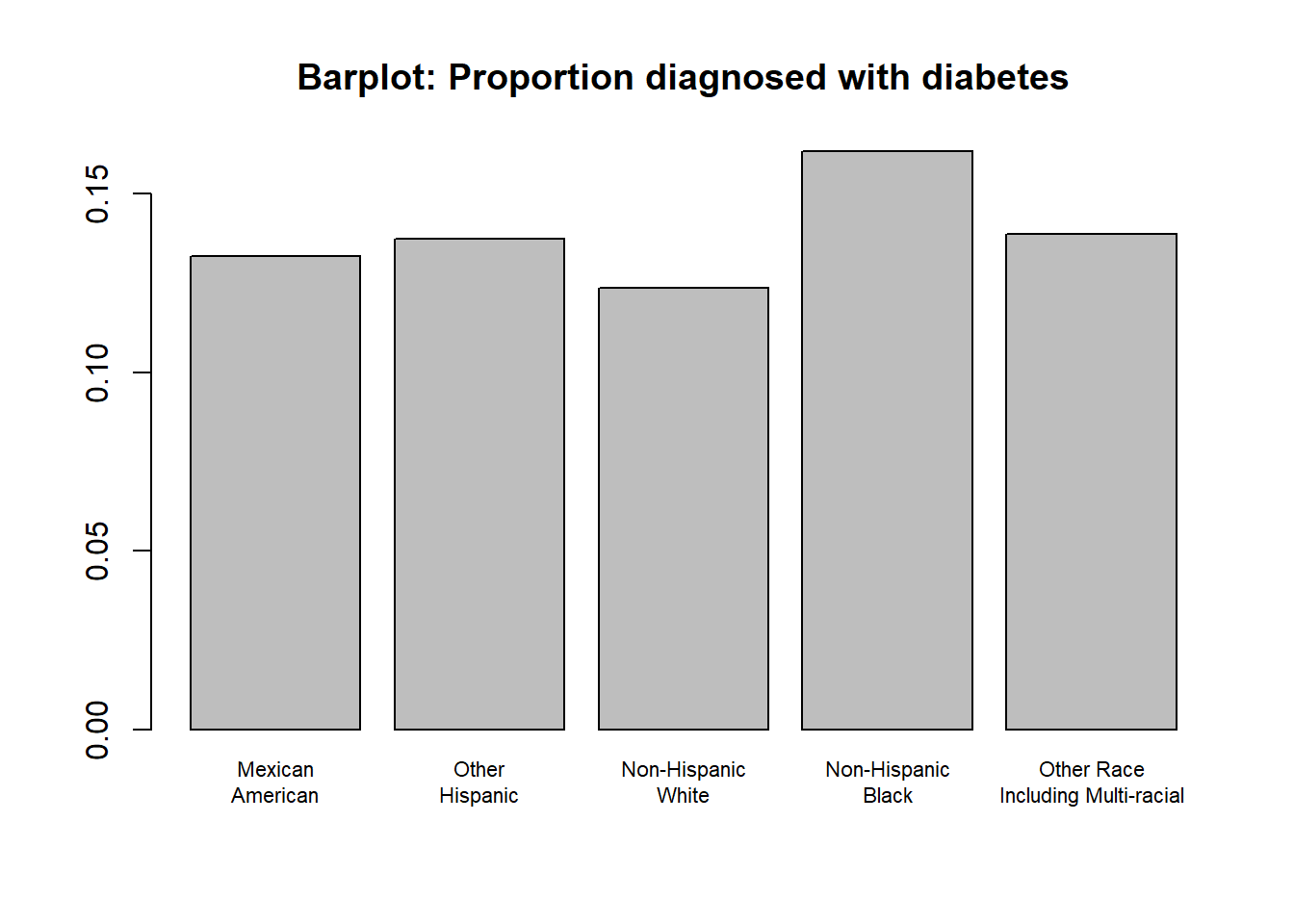
barplot(t1[,"p"],names.arg = t1[,"re"], main ="Barplot: Proportion diagnosed with diabetes", cex.names = .7)
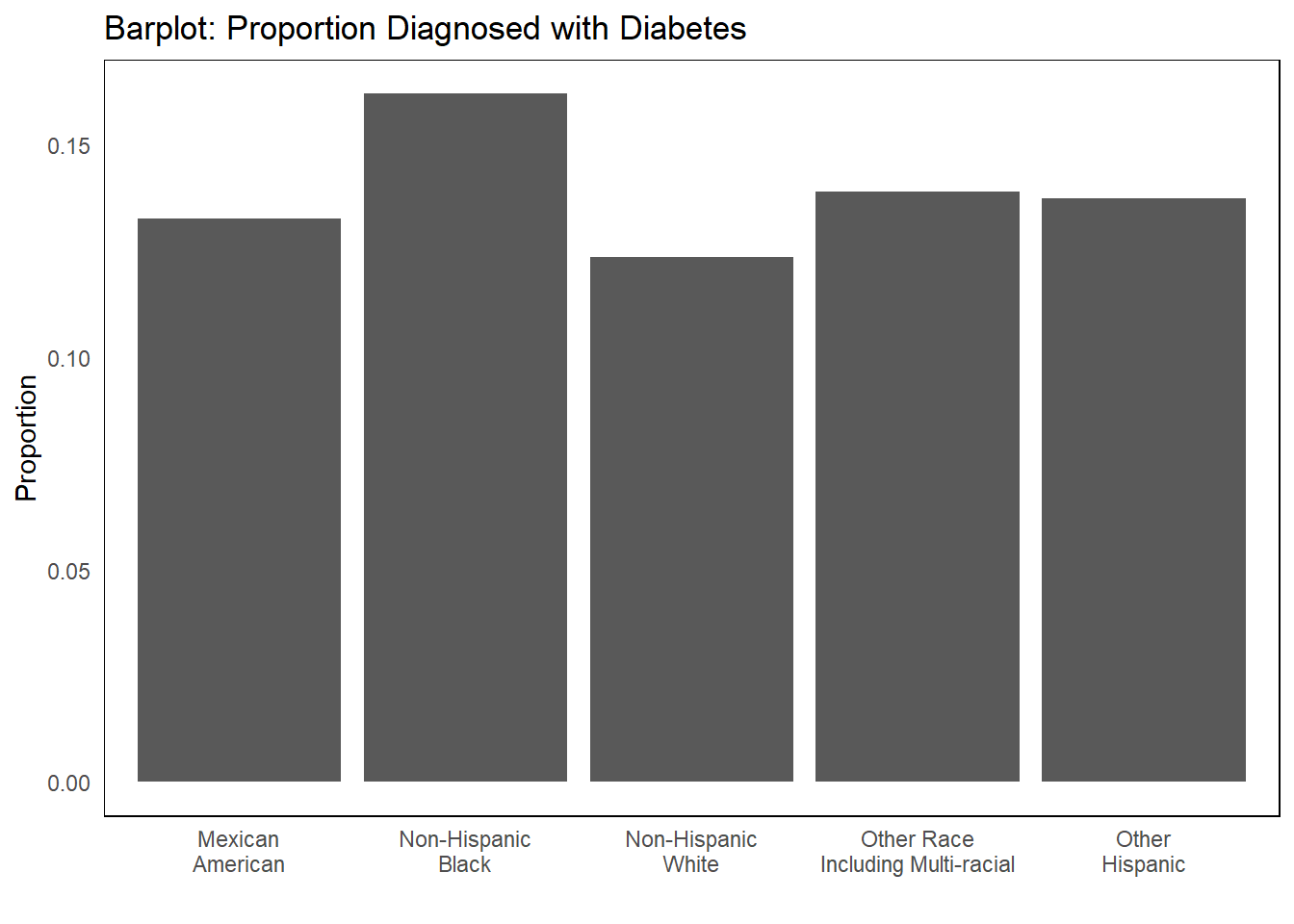
ggplot(t1, aes(x = re, y = p)) +geom_bar(stat ="identity") +labs(title ="Barplot: Proportion Diagnosed with Diabetes", x ="", y ="Proportion") +theme_minimal() +theme(panel.border =element_rect(fill =NA),panel.grid =element_blank() )
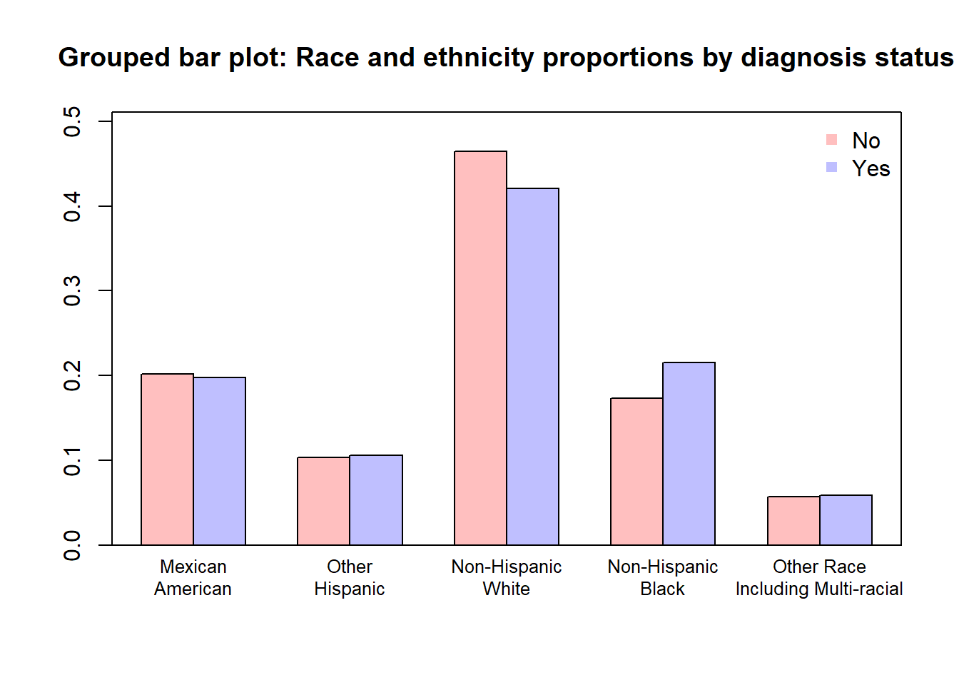
5.3.2.2 Categorical
In this plot, the other conditional proportion is plotted.
t1 <-table(nhgh$dx_f, nhgh$re)m <-rowSums(t1) t2 <- t1/mcolnames(t2) <-colnames(t2) |>gsub(" ", "\n",x=_)colnames(t2)[5] <-"Other Race\nIncluding Multi-racial"cols <-c(rgb(1,0,0,1/4),rgb(0,0,1,1/4))barplot(t2, beside=TRUE, ylim =c(0,max(t2)*1.1), main ="Grouped bar plot: Race and ethnicity proportions by diagnosis status", col = cols, cex.names = .8)box()legend("topright", rownames(t2), pch =15, col = cols, bty ="n")
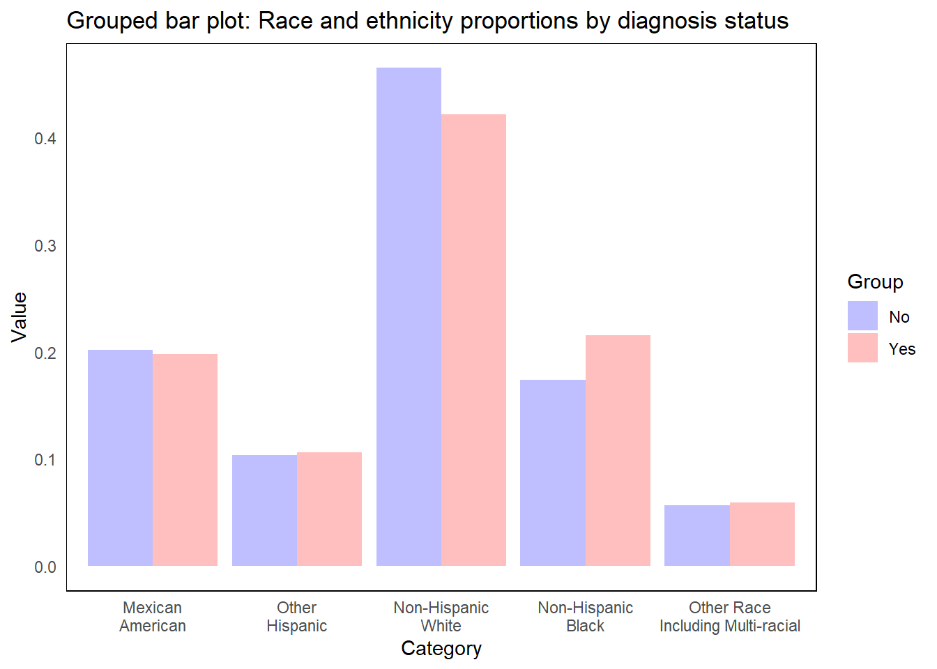
t3 <-as.data.frame(t2)custom_colors <-c("Yes"=rgb(1,0,0,1/4), "No"=rgb(0,0,1,1/4))t3 |>setNames(c("Group","Category","Value")) |>ggplot(aes(x = Category, y = Value, fill = Group)) +geom_bar(stat ="identity", position =position_dodge()) +scale_fill_manual(values = custom_colors) +labs(title="Grouped bar plot: Race and ethnicity proportions by diagnosis status", x ="Category", y ="Value") +theme_minimal() +theme(panel.border =element_rect(fill =NA),panel.grid =element_blank() )